Author: Chen Zhiyan

This article is about 4400 words long and is recommended to read in over 10 minutes. The article provides a detailed interpretation of the source code for the BERT model pre-training task, analyzing each implementation step of the BERT source code in the Eclipse development environment.
The BERT model architecture is an encoder architecture based on multi-layer bidirectional Transformers, released under the tensor2tensor library framework. Due to the use of Transformers in the implementation process, the implementation of the BERT model is almost identical to that of Transformers.
The BERT pre-training model does not use the traditional left-to-right or right-to-left unidirectional language model for pre-training, but instead adopts a bidirectional language model that processes text from both left to right and right to left. This article provides a detailed interpretation of the source code for the BERT model pre-training task, analyzing each implementation step of the BERT source code in the Eclipse development environment.
The code for the BERT model is relatively large, and due to space limitations, it is not possible to explain every line of code. Here, we will explain the function of each core module.
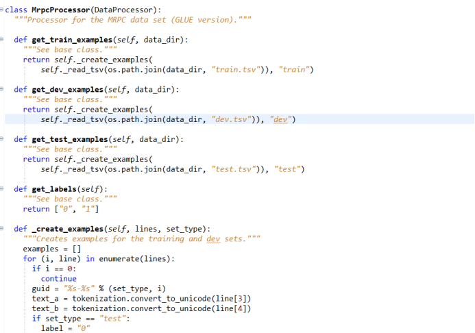
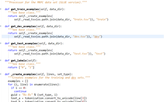
The first step in model training is to read data from the dataset, process it according to the data format required by the BERT model, and write out the specific data processing classes and methods for data processing in the dataset to be used. If the dataset used in the task is not MRPC, this part of the code needs to be rewritten according to the specific task to handle the dataset. For different tasks, a new data reading class needs to be constructed to read the data line by line.
2) Data Preprocessing Module
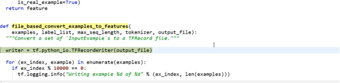
Using TensorFlow to preprocess the data, since reading data in TF-Record format is relatively fast and convenient, it is necessary to convert the data into TF-Record format at the data reading level. First, define a writer, and use the writer function to write the data samples into the TF-Record. This way, during the actual training process, there is no need to read data from the original dataset every time; instead, directly read the processed data from the TF-Record.
The specific method for converting each data sample into TF-Record format is as follows: First, construct a label, then judge how many sentences are composed in the data, take the current first sentence, and perform a tokenization operation. The tokenization method is the wordpiece method. In English text, words are composed of letters, and words are separated by spaces. Simply separating words by spaces is often insufficient, so further segmentation of words is needed. In the BERT model, the wordpiece method is called to further segment the input words, using the greedy matching method of wordpiece to break the input words into subwords, enriching the meaning expressed by the words. Here, the wordpiece method is used to further segment the input words, breaking the input word sequence into more basic units, making it easier for the model to learn.
In the Chinese system, sentences are usually segmented into individual characters. After segmentation, the input is transformed into the wordpiece structure using wordpiece. Then, a judgment is made to see if there is a second sentence input. If there is a second sentence input, the same processing is performed using wordpiece. After completing the wordpiece transformation, a judgment is made to determine whether the actual sentence length exceeds the value of max_seq_length. If the length of the input sentence exceeds the specified value of max_seq_length, truncation is required.
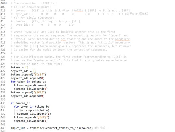
Encoding the input sentence pairs, traversing each word in the wordpiece structure and its corresponding type_id, adding sentence separators [CLS], [SEP], and adding encoding information for all results; adding type_id, mapping all words to index functions, and encoding the ID (identifier) of input words for easy lookup during subsequent word embedding;
Mask encoding: For sentences shorter than max_seq_length, padding is performed. In the calculation of self-attention, only the actual words in the sentence are considered. The input_mask operation is performed on the input sequence, adding additional masks for positions with fewer than 128 words, to inform self-attention to only compute the actual words. During subsequent self-attention calculations, words with input_mask=0 will be ignored, and only words with input_mask=1 will participate in the self-attention calculation. Mask encoding initializes the preprocessing of task data for subsequent fine-tuning operations.
Initializing input_Feature: Constructing input_Feature and returning the result to BERT. Using a for loop to traverse each sample, converting input_id, input_mask, and segment_id to int type for the subsequent creation of TF-Record. The reason for this data type conversion is that the official TensorFlow API requires it; TensorFlow has strict regulations on the format of TF-Record that cannot be modified by users. In subsequent specific project tasks, when creating TF-Record, simply copy all the original code over and modify it according to the original format. After constructing the input_Feature, pass it to tf_example, convert it to tf_train_features, and then write it into the constructed data.
4) Role of the Embedding Layer
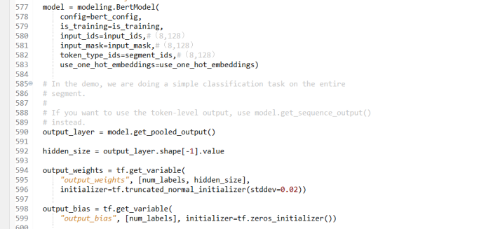
In the BERT model, there is a create_model function, which constructs the model step by step. First, create a BERT model that contains all the structures of the transformer, as follows:
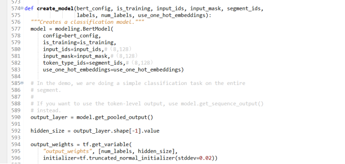
Read the configuration file, determine whether training is required, and read in variables such as input_id, input_mask, and segment_id. The one_hot_embedding variable is only used when training with TPU and is not considered when training with CPU, with the default value set to false.
Construct the embedding layer, i.e., word embedding. The word embedding operation converts the current sequence into vectors. The embedding layer of BERT must consider not only the input word sequence but also other additional information and positional information. The word embedding vector constructed by BERT contains the following three types of information: the input word sequence information, other additional information, and positional information. To perform calculations between vectors, it is necessary to keep the dimensions of the word vectors containing these three types of information consistent.
5) Adding Additional Encoding Features
Next, we enter the embedding_lookup layer. The input to this layer includes: input_id (input identifier), vocab_size (size of the vocabulary), embedding_size (dimension of the word embedding), and initializer_range (range of initialization values). The output of embedding_lookup is an actual vector encoding.
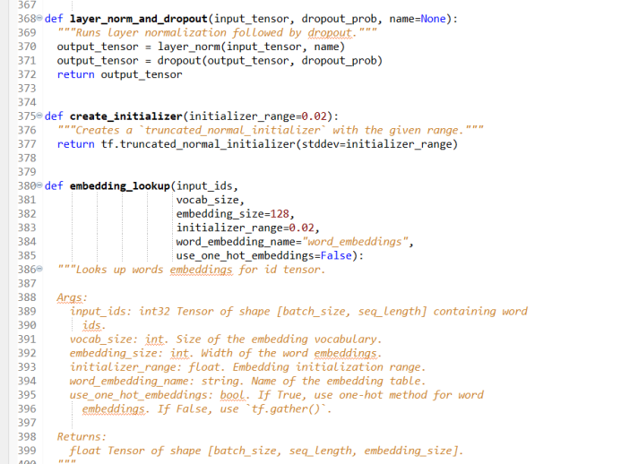
First, obtain the embedding_table, then look up the word vector corresponding to each word in the embedding_table and return the final result to output. In this way, the input words become word vectors. However, this operation is only part of the word embedding; a complete word embedding should also add other additional information in the word embedding, namely: embedding_post_processor.
embedding_post_processor is the second part of the information that must be added to the word embedding operation. The inputs to embedding_post_processor include: input_tensor, use_token_type, token_type_id, token_type_vocab_size, and the returned feature vector will contain this additional information, with dimensions consistent with the input word vectors.
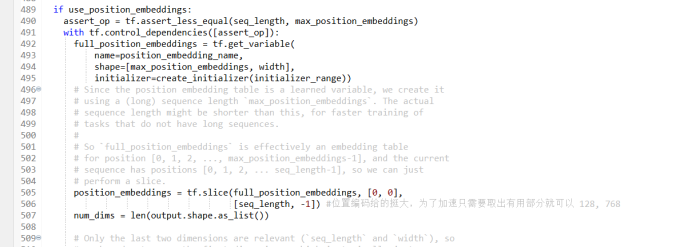
6) Adding Positional Encoding Features
Using use_position_embedding to add positional encoding information. The self-attention in BERT needs to include positional encoding information. First, initialize positional encoding with full_position_embedding, adding the positional encoding vector of each word to the word embedding vector. Then, perform a calculation based on the current sequence length. If the sequence length is 128, the positional encoding is performed for these 128 positions. Since positional encoding contains only positional information and is unrelated to the semantic context of the sentence, the positional encoding results are the same for different input sequences. Regardless of the content of the input sequences, their positional encodings are the same. After obtaining the output results of positional encoding, the additional encoding features obtained are added to the original word embedding output vector, and the three vectors are summed to return the summation result. At this point, the input word embedding of the BERT model is completed, resulting in a word vector that contains positional information, which will undergo further operations.
After completing the word embedding, the next step is the Transformer structure. Before the Transformer, some transformations need to be performed on the word vectors, namely attention_mask, creating a mask matrix: create_attention_mask_from_input_mask. In the previously mentioned input_mask, only words with mask=1 participate in the calculation of attention. Now, this two-dimensional mask needs to be converted into a three-dimensional mask, indicating which word vectors will participate in the actual calculation when entering attention. That is, in the calculation of attention, which words among the 128 words in the input sequence will do attention calculations. Here, an additional mask processing operation is added.
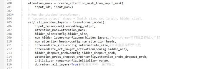
After completing the mask processing, the next step is to construct the encoding side of the Transformer. First, some parameters such as input_tensor, attention_mask, hidden_size, head_num, etc., are passed to the Transformer. These parameters have already been set during the pre-training process and should not be changed arbitrarily during fine-tuning operations.
In the multi-head attention mechanism, each head generates a feature vector, and finally, the vectors generated by each head are concatenated together to obtain the output feature vector.
8) Constructing QKV Matrices
The next step is the implementation of the attention mechanism. The attention mechanism in BERT is a multi-layered architecture. In the specific implementation, a traversal operation is used to achieve the stacking of multiple layers. A total of 12 layers need to be traversed, where the input of the current layer is the output of the previous layer. In the attention mechanism, two vectors are input: from-tensor and to_tensor, while BERT’s attention mechanism uses self_attention, at this time:
from-tensor=to_tensor=layer_input;
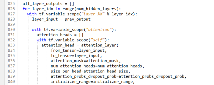
In constructing the attention_layer, it is necessary to construct the K, Q, V matrices, which are the core parts of the transformer. When constructing the K, Q, V matrices, the following abbreviations will be used:
-
B represents Batch Size, typically set to 8;
-
F represents from-tensor, with a dimension of 128;
-
T represents to_tensor, with a dimension of 128;
-
N represents the Number of Attention Heads (multi-head attention mechanism), typically set to 12 heads;
-
H represents Size_per_head, indicating how many feature vectors each head contains, typically set to 64;
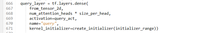
Constructing the Query matrix: The query_layer is constructed from the from-tensor. In the multi-head attention mechanism, the number of attention heads generates the same number of Query matrices, with each head generating a corresponding output vector:
query_layer=[B*F,N*H], i.e., 1024*768;
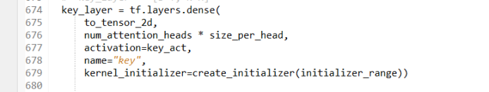
Constructing the Key matrix: The Key matrix is constructed from the to-tensor. In the multi-head attention mechanism, the number of attention heads generates the same number of Key matrices, with each head generating a corresponding output vector:
key_layer=[B*T,N*H], i.e., 1024*768;
Constructing the Value matrix: The construction of the Value matrix is similar to that of the Key matrix, differing only in the description:
value_layer=[B*T,N*H], i.e., 1024*768;
After constructing the QKV matrices, calculate the inner product of the K matrix and the Q matrix, and then perform a Softmax operation. The Value matrix helps us understand the actual features obtained, and the Value matrix corresponds exactly to the Key matrix, with identical dimensions.
9) Completing the Construction of the Transformer Module
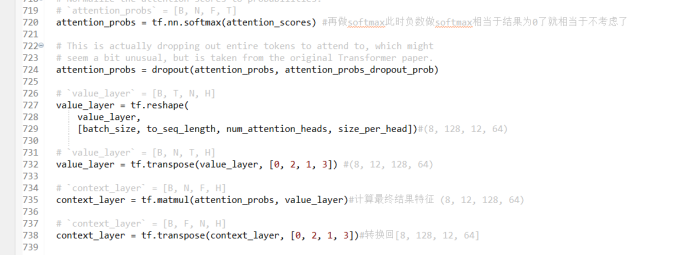
After constructing the QKV matrices, the next step is to calculate the inner product of the K matrix and the Q matrix. To speed up the calculation of the inner product, a transpose conversion is performed here to accelerate the calculation without affecting subsequent operations. After calculating the inner product of the K matrix and the Q matrix, the attention score is obtained: attention_score. Finally, the Softmax operation is used to convert the obtained attention scores into probabilities: attention_prob.
Before performing the Softmax operation, to reduce the computational load, an attention_mask is added to mask out the words in the sequence of length 128 that are not actual words, preventing them from participating in the calculation. In TensorFlow, there is a ready-made Softmax function that can be called. By passing all the current attention scores into Softmax, the result obtained is a probability value, which is used as a weight and combined with the Value matrix. That is, the attention_prob and Value matrix are multiplied together to obtain the context semantic matrix:
Context_layer=tf.matmul(attention_prob, value_layer);

After obtaining the output of the current layer’s context semantic matrix, this output serves as the input for the next layer, participating in the attention calculations of the next layer. The multi-layer attention is achieved through multiple iterations using a for loop. The number of iterations corresponds to the number of attention layers (in this case, 12 layers).
10) Training the BERT Model
After completing the self-attention, the next step is a fully connected layer. Here, it is necessary to consider the fully connected layer, using tf.layer.dense to implement a fully connected layer, and finally performing a residual connection. Note: In the implementation of the fully connected layer, the final result must be returned, that is, the output of the last attention layer is returned to BERT, which is the entire structure of the Transformer.
To summarize the entire process described above, the implementation of the Transformer mainly consists of two parts: the first part is the embedding layer, which combines the wordpiece embeddings with additional specific information and positional encoding information, resulting in the output vector of the embedding layer; the second part is sending the output vector of the embedding layer into the transformer structure, constructing the K, Q, V matrices, and using the Softmax function to obtain the context semantic matrix C. The context semantic matrix C not only contains the encoding features of each word in the input sequence but also includes the positional encoding information of each word.
This is the implementation method of the BERT model. Understanding the detailed process of these two major parts will clarify any major issues with understanding the BERT model. The ten steps above cover the important operations in the BERT model.
After the BERT model, the final result obtained is a feature vector representing the final outcome. This is the entire process of the open-source MRPC project officially published by Google. When readers construct their specific task projects, the part of the code that needs to be modified is how to read data into the BERT model and implement data preprocessing.
Introduction to the DataPi Research Department
Established in early 2017, the DataPi Research Department is divided into multiple groups centered around interests. Each group adheres to the overall principles of knowledge sharing and project planning, while also having its own unique characteristics:
Algorithm Model Group: Actively participates in Kaggle and other competitions, producing original hands-on tutorial articles;
Research and Analysis Group: Investigates the applications of big data through interviews and explores the beauty of data products;
System Platform Group: Tracks cutting-edge technologies in big data and AI system platforms, engaging with experts;
Natural Language Processing Group: Focuses on practical applications, actively participating in competitions and planning various text analysis projects;
Manufacturing Big Data Group: Pursues the dream of becoming a strong industrial nation, integrating industry, academia, research, and government to unlock data value;
Data Visualization Group: Merges information and art to explore the beauty of data, learning to tell stories through visualization;
Web Scraping Group: Gathers information from the web, collaborating with other groups to develop creative projects.
Click on the end of the article “Read the Original” to sign up as a DataPi Research Department Volunteer, there’s bound to be a group that suits you~
Reprint Notice
If you need to reprint, please prominently indicate the author and source at the beginning of the article (originally from: DataPi THU ID: DatapiTHU), and place a prominent QR code for DataPi at the end of the article. For articles with original identification, please send [Article Title – Pending Authorized Official Account Name and ID] to the contact email to apply for whitelist authorization and edit as required.
Unauthorized reprints and adaptations will be legally pursued.

Click “Read the Original” to join the organization~