
Hello everyone, I am Redstone!
In the previous article:
Implementing VGGNet (Theoretical Part)
We detailed the network structure of VGGNet. Today, we will use PyTorch to reproduce the VGGNet network and apply the VGGNet model to solve a classic Kaggle image recognition competition problem.
Let’s get started!
1. Dataset Preparation
In the paper, the authors of AlexNet used the ILSVRC 2012 competition dataset, which is very large (138G), and downloading and training it is time-consuming. Therefore, we will not use this dataset for our reproduction. Since datasets like MNIST, CIFAR10, and CIFAR100 have smaller image sizes that do not meet the input size requirement of 227×227 for the AlexNet network, we will use the classic “Dogs vs. Cats” dataset from Kaggle instead.
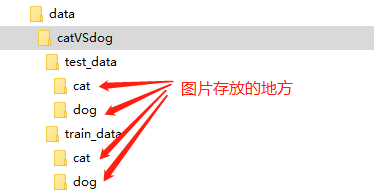
This dataset contains a total of 25,000 training images, with 12,500 cats and 12,500 dogs, all labeled; the test set contains 12,500 images without labels. We will only use the labeled 25,000 images, taking out 2,500 images of cats and dogs respectively as the validation set for the model. We will organize the dataset images according to the following directory structure.
To facilitate training, we have placed this dataset on Baidu Cloud, download link:
Link: https://pan.baidu.com/s/1UEOzxWWMLCUoLTxdWUkB4A
Extraction Code: cdue
1.1 Creating Image Data Index
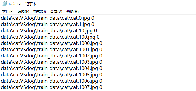
Once the dataset is prepared, we need to read it using PyTorch and create a dataset that can be used for training and testing. For both the training and testing sets, we first need to create corresponding image data indices, namely train.txt and test.txt files. Each txt file contains the directory of each image and the corresponding class (cat corresponds to label=0, dog corresponds to label=1). The schematic is as follows:
The Python script to create the image data indices train.txt and test.txt is as follows:
import os

train_txt_path = os.path.join("data", "catVSdog", "train.txt")
train_dir = os.path.join("data", "catVSdog", "train_data")
valid_txt_path = os.path.join("data", "catVSdog", "test.txt")
valid_dir = os.path.join("data", "catVSdog", "test_data")

def gen_txt(txt_path, img_dir):
    f = open(txt_path, 'w')

    for root, s_dirs, _ in os.walk(img_dir, topdown=True):  # Get folder names under train
        for sub_dir in s_dirs:
            i_dir = os.path.join(root, sub_dir)             # Get absolute path of each category folder
            img_list = os.listdir(i_dir)                    # Get paths of all png images under the category folder
            for i in range(len(img_list)):
                if not img_list[i].endswith('jpg'):         # If not a png file, skip
                    continue
                #label = (img_list[i].split('.')[0] == 'cat')? 0 : 1
                label = img_list[i].split('.')[0]
                # Convert character category to integer type
                if label == 'cat':
                    label = '0'
                else:
                    label = '1'
                img_path = os.path.join(i_dir, img_list[i])
                line = img_path + ' ' + label + '\n'
                f.write(line)
    f.close()

if __name__ == '__main__':
    gen_txt(train_txt_path, train_dir)
    gen_txt(valid_txt_path, valid_dir)
After running the script, train.txt and test.txt index files will be generated in the ./data/catVSdog/ directory.
1.2 Building the Dataset Subclass
To load our dataset in PyTorch, we need to write a class that inherits from torch.utils.data’s Dataset and modify its __init__, __getitem__, and __len__ methods. The default loading is for images, and the purpose of __init__ is to get a list containing data and labels, where each element can locate the image and its corresponding label. Then use __getitem__ to get the image pixel matrix and label for each element, returning img and label.
from PIL import Image
from torch.utils.data import Dataset

class MyDataset(Dataset):
    def __init__(self, txt_path, transform = None, target_transform = None):
        fh = open(txt_path, 'r')
        imgs = []
        for line in fh:
            line = line.rstrip()
            words = line.split()
            imgs.append((words[0], int(words[1]))) # Convert category to int
            self.imgs = imgs
            self.transform = transform
            self.target_transform = target_transform
    def __getitem__(self, index):
        fn, label = self.imgs[index]
        img = Image.open(fn).convert('RGB')
        #img = Image.open(fn)
        if self.transform is not None:
            img = self.transform(img)
        return img, label
    def __len__(self):
        return len(self.imgs)
getitem is the core function. self.imgs is a list, where self.imgs[index] is a string containing the image path and label, which is read from the generated txt file; using Image.open to read the image, noting whether the img is single-channel or three-channel; self.transform(img) processes the image, where this transform can implement mean subtraction, standard deviation division, random cropping, rotation, flipping, affine transformation, etc.
1.3 Loading the Dataset and Data Preprocessing
Once MyDataset is built, the remaining operations are left to DataLoader to load the dataset. In DataLoader, the getitem function in MyDataset will be triggered to read the data and label of one image, and concatenate them into a batch to return as the actual input to the model.
pipline_train = transforms.Compose([
    #transforms.RandomResizedCrop(224),
    transforms.RandomHorizontalFlip(),  # Randomly flip the image horizontally
    # Resize the image to 224x224
    transforms.Resize((224,224)),
    # Convert the image to Tensor format
    transforms.ToTensor(),
    # Normalization (used to reduce model complexity when overfitting occurs)
    transforms.Normalize((0.5, 0.5, 0.5), (0.5, 0.5, 0.5))
    #transforms.Normalize(mean = [0.485, 0.456, 0.406],std = [0.229, 0.224, 0.225])
])
pipline_test = transforms.Compose([
    # Resize the image to 224x224
    transforms.Resize((224,224)),
    transforms.ToTensor(),
    transforms.Normalize((0.5, 0.5, 0.5), (0.5, 0.5, 0.5))
    #transforms.Normalize(mean = [0.485, 0.456, 0.406],std = [0.229, 0.224, 0.225])
])
train_data = MyDataset('./data/catVSdog/train.txt', transform=pipline_train)
test_data = MyDataset('./data/catVSdog/test.txt', transform=pipline_test)

# train_data and test_data contain all training and testing data, call DataLoader for batch loading
trainloader = torch.utils.data.DataLoader(dataset=train_data, batch_size=64, shuffle=True)
testloader = torch.utils.data.DataLoader(dataset=test_data, batch_size=32, shuffle=False)
# Class information also needs to be given
classes = ('cat', 'dog') # Corresponding to label=0, label=1
In data preprocessing, we adjust the image size to 224×224, meeting the input requirements of the VGGNet network. Mean = [0.5, 0.5, 0.5], variance = [0.5, 0.5, 0.5], and then use transforms.Normalize for normalization.
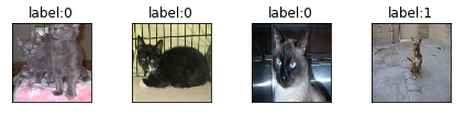
Now, let’s take a look at the final dataset images and their corresponding labels:
examples = enumerate(trainloader)
batch_idx, (example_data, example_label) = next(examples)
# Batch display images
for i in range(4):
    plt.subplot(1, 4, i + 1)
    plt.tight_layout()  # Automatically adjust subplot parameters to fill the entire image area
    img = example_data[i]
    img = img.numpy() # Convert FloatTensor to ndarray
    img = np.transpose(img, (1,2,0)) # Move the channel dimension to the last
    img = img * [0.5, 0.5, 0.5] + [0.5, 0.5, 0.5]
    #img = img * [0.229, 0.224, 0.225] + [0.485, 0.456, 0.406]
    plt.imshow(img)
    plt.title("label:{}'.format(example_label[i]))
    plt.xticks([])
    plt.yticks([])
plt.show()
2. Building the VGGNet Neural Network Structure
class VGG(nn.Module):
    def __init__(self, features, num_classes=2, init_weights=False):
        super(VGG, self).__init__()
        self.features = features
        self.classifier = nn.Sequential(
            nn.Linear(512*7*7, 500),
            nn.ReLU(True),
            nn.Dropout(p=0.5),
            nn.Linear(500, 20),
            nn.ReLU(True),
            nn.Dropout(p=0.5),
            nn.Linear(20, num_classes)
        )
        if init_weights:
            self._initialize_weights()

    def forward(self, x):
        # N x 3 x 224 x 224
        x = self.features(x)
        # N x 512 x 7 x 7
        x = torch.flatten(x, start_dim=1)
        # N x 512*7*7
        x = self.classifier(x)
        return x

    def _initialize_weights(self):
        for m in self.modules():
            if isinstance(m, nn.Conv2d):
                # nn.init.kaiming_normal_(m.weight, mode='fan_out', nonlinearity='relu')
                nn.init.xavier_uniform_(m.weight)
                if m.bias is not None:
                    nn.init.constant_(m.bias, 0)
            elif isinstance(m, nn.Linear):
                nn.init.xavier_uniform_(m.weight)
                # nn.init.normal_(m.weight, 0, 0.01)
                nn.init.constant_(m.bias, 0)


def make_features(cfg: list):
    layers = []
    in_channels = 3
    for v in cfg:
        if v == "M":
            layers += [nn.MaxPool2d(kernel_size=2, stride=2)]
        else:
            conv2d = nn.Conv2d(in_channels, v, kernel_size=3, padding=1)
            layers += [conv2d, nn.ReLU(True)]
            in_channels = v
    return nn.Sequential(*layers)


cfgs = {
    'vgg11': [64, 'M', 128, 'M', 256, 256, 'M', 512, 512, 'M', 512, 512, 'M'],
    'vgg13': [64, 64, 'M', 128, 128, 'M', 256, 256, 'M', 512, 512, 'M', 512, 512, 'M'],
    'vgg16': [64, 64, 'M', 128, 128, 'M', 256, 256, 256, 'M', 512, 512, 512, 'M', 512, 512, 512, 'M'],
    'vgg19': [64, 64, 'M', 128, 128, 'M', 256, 256, 256, 256, 'M', 512, 512, 512, 512, 'M', 512, 512, 512, 512, 'M'],
}


def vgg(model_name="vgg16", **kwargs):
    assert model_name in cfgs, "Warning: model number {} not in cfgs dict!".format(model_name)
    cfg = cfgs[model_name]

    model = VGG(make_features(cfg), **kwargs)
    return model
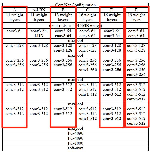
First, we selected four structures A, B, D, and E from the six VGG structures to build the model. The cfg dictionary created contains these four structures. For example, for vgg16, [64, 64, ‘M’, 128, 128, ‘M’, 256, 256, 256, ‘M’, 512, 512, 512, ‘M’, 512, 512, 512, ‘M’] represents the structure of the convolutional layers. 64 means conv3-64, ‘M’ means maxpool, 128 means conv3-128, 256 means conv3-256, and 512 means conv3-512.
Once the VGG structure is determined, the list is passed into the make_features() function to build the convolutional layers of VGG, and the function returns an instantiated model. For example, let’s construct the convolutional layer structure of vgg16 and print it:
cfg = cfgs['vgg16']
make_features(cfg)
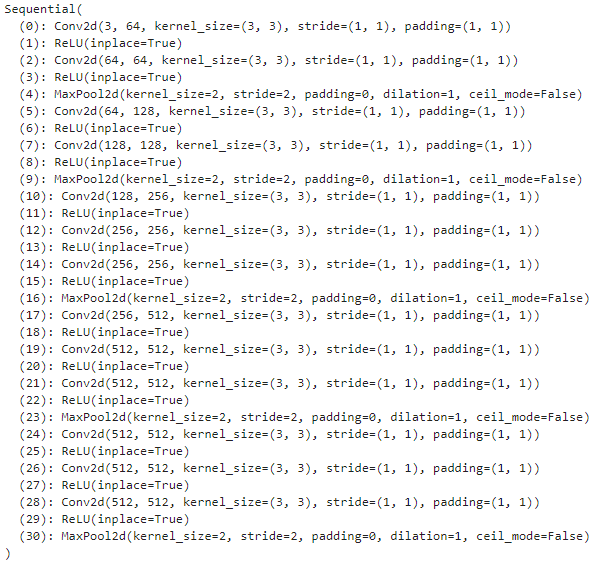
When defining the VGG class, the parameter num_classes refers to the number of classes. Since our dataset has only two categories, cats and dogs, the number of neurons in the fully connected layer has been adjusted. num_classes=2, and the output layer has only two neurons instead of the original 1000 neurons. FC4096 has been adjusted from the original 4096 neurons to 500 and 20 neurons respectively. Please note this adjustment based on the actual number of classes in your dataset. The rest of the network structure is exactly the same as in the paper.
The function initialize_weights() performs the parameter initialization operation for the network; we default to disabling the initialization operation.
The forward() function defines the complete structure of the VGG network. Note that the output feature map from the last convolutional layer is N x 512 x 7 x 7, where N represents the batch size, and it needs to be flattened into a one-dimensional vector to facilitate connection with the fully connected layer.
3. Deploying the Defined Network Structure to GPU/CPU and Defining the Optimizer
# Create model, deploy to GPU
device = torch.device("cuda" if torch.cuda.is_available() else "cpu")
model_name = "vgg16"
model = vgg(model_name=model_name, num_classes=2, init_weights=True)
model.to(device)
# Define optimizer
loss_function = nn.CrossEntropyLoss()
optimizer = optim.Adam(model.parameters(), lr=0.0001)
4. Defining the Training Process
def train_runner(model, device, trainloader, loss_function, optimizer, epoch):
    # Train the model, enable BatchNormalization and Dropout, set BatchNormalization and Dropout to True
    model.train()
    total = 0
    correct =0.0

    # Enumerate through the loaded dataset while getting data and index
    for i, data in enumerate(trainloader, 0):
        inputs, labels = data
        # Deploy the model to the device
        inputs, labels = inputs.to(device), labels.to(device)
        # Initialize gradients
        optimizer.zero_grad()
        # Save training results
        outputs = model(inputs)
        # Calculate loss
        #loss = F.cross_entropy(outputs, labels)
        loss = loss_function(outputs, labels)
        # Get the predicted results with the highest probability
        # dim=1 means return the index of the maximum value for each row
        predict = outputs.argmax(dim=1)
        total += labels.size(0)
        correct += (predict == labels).sum().item()
        # Backpropagation
        loss.backward()
        # Update parameters
        optimizer.step()
        if i % 100 == 0:
            # loss.item() indicates the current loss value
            print("Train Epoch{} \t Loss: {:.6f}, accuracy: {:.6f}%".format(epoch, loss.item(), 100*(correct/total)))
            Loss.append(loss.item())
            Accuracy.append(correct/total)
    return loss.item(), correct/total
5. Defining the Testing Process
def test_runner(model, device, testloader):
    # Model validation, must be written; otherwise, as long as there is input data, even if not trained, it will change weights
    # Calling eval() will disable BatchNormalization and Dropout, setting BatchNormalization and Dropout to False
    model.eval()
    # Count model accuracy, initial value set
    correct = 0.0
    test_loss = 0.0
    total = 0
    # torch.no_grad will not calculate gradients and will not perform backpropagation
    with torch.no_grad():
        for data, label in testloader:
            data, label = data.to(device), label.to(device)
            output = model(data)
            test_loss += F.cross_entropy(output, label).item()
            predict = output.argmax(dim=1)
            # Calculate correct count
            total += label.size(0)
            correct += (predict == label).sum().item()
        # Calculate loss value
        print("test_average_loss: {:.6f}, accuracy: {:.6f}%".format(test_loss/total, 100*(correct/total)))
6. Running the Model
# Call
epoch = 20
Loss = []
Accuracy = []
for epoch in range(1, epoch+1):
    print("start_time",time.strftime('%Y-%m-%d %H:%M:%S',time.localtime(time.time())))
    loss, acc = train_runner(model, device, trainloader, loss_function, optimizer, epoch)
    Loss.append(loss)
    Accuracy.append(acc)
    test_runner(model, device, testloader)
    print("end_time: ",time.strftime('%Y-%m-%d %H:%M:%S',time.localtime(time.time())),'\n')

print('Finished Training')
plt.subplot(2,1,1)
plt.plot(Loss)
plt.title('Loss')
plt.show()
plt.subplot(2,1,2)
plt.plot(Accuracy)
plt.title('Accuracy')
plt.show()
After 20 epochs of training, the accuracy reached 94.68%.
Note that due to the large size of the VGGNet network, running on CPU can be very slow or even freeze; it is recommended to train using GPU.
7. Saving the Model
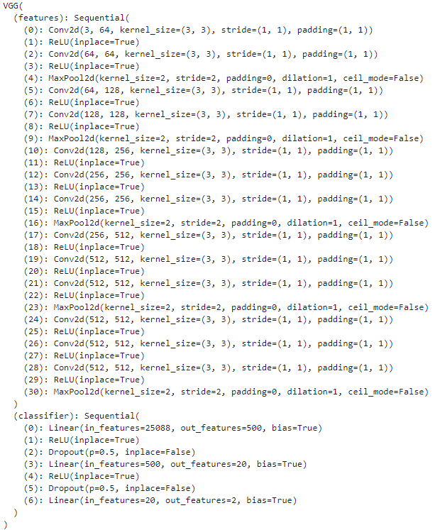
print(model)
torch.save(model, './models/vgg-catvsdog.pth') # Save model
The VGGNet model will be printed out, and the model will be saved as vgg-catvsdog.pth in a fixed directory.
8. Model Testing
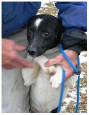
Now we will test the model using an image from the Dogs vs. Cats test set.
from PIL import Image
import numpy as np

if __name__ == '__main__':
    device = torch.device('cuda' if torch.cuda.is_available() else 'cpu')
    model = torch.load('./models/vgg-catvsdog.pth') # Load model
    model = model.to(device)
    model.eval()    # Set model to test mode

    # Read the image to be predicted
    img = Image.open("./images/test_dog.jpg") # Read image
    #img.show()
    plt.imshow(img) # Display image
    plt.axis('off') # Do not show axis
    plt.show()

    # Import image, resized to [1,1,32,32]
    trans = transforms.Compose(
        [
            transforms.Resize((227,227)),
            transforms.ToTensor(),
            transforms.Normalize((0.5, 0.5, 0.5), (0.5, 0.5, 0.5))
            #transforms.Normalize(mean = [0.485, 0.456, 0.406],std = [0.229, 0.224, 0.225])
        ])
    img = trans(img)
    img = img.to(device)
    img = img.unsqueeze(0)  # Extend the image to one more dimension, because input to the saved model is 4D [batch_size, channels, height, width], while normal images are only 3D [channels, height, width]

    # Prediction
    # Prediction
    classes = ('cat', 'dog')
    output = model(img)
    prob = F.softmax(output,dim=1) # prob is the probabilities of the two categories
    print("Probability:",prob)
    value, predicted = torch.max(output.data, 1)
    predict = output.argmax(dim=1)
    pred_class = classes[predicted.item()]
    print("Predicted class:",pred_class)
Output:
Probability: tensor([[7.6922e-08, 1.0000e+00]], device=’cuda:0′, grad_fn=<SoftmaxBackward>)
Predicted class: dog
The model prediction result is correct!
That’s it! This is the core code for reproducing the VGGNet network using PyTorch. I recommend that everyone code along with the article and use your own dataset with appropriate adjustments to the network structure.
The complete code has been placed on GitHub, link:
https://github.com/RedstoneWill/CNN_PyTorch_Beginner/blob/main/VGGNet/VGGNet.ipynb
Hand-Crafted CNN Series:
Hand-Crafted CNN Classic Network: LeNet-5 (Theoretical Part)
Hand-Crafted CNN Classic Network: LeNet-5 (MNIST Practical Part)
Hand-Crafted CNN Classic Network: LeNet-5 (CIFAR10 Practical Part)
Hand-Crafted CNN Classic Network: LeNet-5 (Custom Practical Part)
Hand-Crafted CNN Classic Network: AlexNet (Theoretical Part)
Hand-Crafted CNN Classic Network: AlexNet (PyTorch Practical Part)
Hand-Crafted CNN Classic Network: VGGNet (Theoretical Part)
If you find this article useful, please give it a thumbs up or share it with your friends!
Recommended Reading
(Click the title to jump to read)
Essentials | Selected Historical Articles from Public Accounts
My Deep Learning Entry Route
My Machine Learning Entry Roadmap
Important!
The annual technical article electronic version PDF from AI has arrived!
Scan the QR code below to add AI’s assistant WeChat, apply to join the group, and obtain the complete collection of technical articles from 2020 PDF (please be sure to note:Join + Location + School/Company. For example:Join+Shanghai+Fudan.

Long press to scan and apply to join the group
(Due to a large number of applicants, please be patient)