Selected from arXiv
Translated by Machine Heart
Contributors: Huang Xiaotian, Lu Xue, Jiang Siyuan
Recently, researchers from Nanyang Technological University published a paper describing the mathematical principles of convolutional networks. This paper explains the entire operation and propagation process of convolutional networks from a mathematical perspective. It is very helpful for understanding the mathematical essence of convolutional networks, assisting readers in implementing convolutional networks “from scratch” (without using convolution APIs).
Paper link: https://arxiv.org/pdf/1711.03278.pdf
In this paper, we will explore the mathematical essence of convolutional networks from aspects such as convolution architecture, constituent modules, and propagation processes. Readers may already be familiar with the specific operational processes of convolutional networks. Beginners can first refer to the first part of the Capsule paper interpretation to understand the detailed convolution process. However, we generally do not focus on how convolutional networks are implemented mathematically. Since major deep learning frameworks provide concise convolution layer APIs, we can construct various convolution layers without needing mathematical expressions; we only need to focus on the tensor dimensions of the input and output of convolution operations. While this allows us to implement networks perfectly, our understanding of the mathematical essence and processes of convolutional networks remains unclear, which is the purpose of this paper.
Below, we will briefly introduce the main content of this paper and attempt to understand the mathematical processes of convolutional networks. Readers with a foundation can refer to the original paper for a deeper understanding. Additionally, we may be able to implement a simple convolutional network without using hierarchical APIs by leveraging the computational formulas from this paper.
Convolutional Neural Networks (CNNs), also known as ConvNets, are widely used in many visual image and speech recognition tasks. After Alex Krizhevsky and others first applied deep convolutional networks in the 2012 ImageNet Challenge, the architectural design of deep convolutional neural networks has attracted many researchers’ contributions. This has significantly impacted the construction of deep learning architectures, such as TensorFlow, Caffe, Keras, and MXNet. Although deep learning implementations can be easily completed through frameworks, the mathematical theories and concepts are very difficult for beginners and practitioners to understand. This paper will attempt to outline the architecture of convolutional networks and explain the mathematical derivation involving activation functions, loss functions, forward propagation, and backward propagation. In this paper, we use grayscale images as input information, ReLU and Sigmoid activation functions to construct the non-linear properties of convolutional networks, and the cross-entropy loss function to calculate the distance between predicted values and true values. This convolutional network architecture includes a convolution layer, pooling layer, and multiple fully connected layers.
2 Architecture
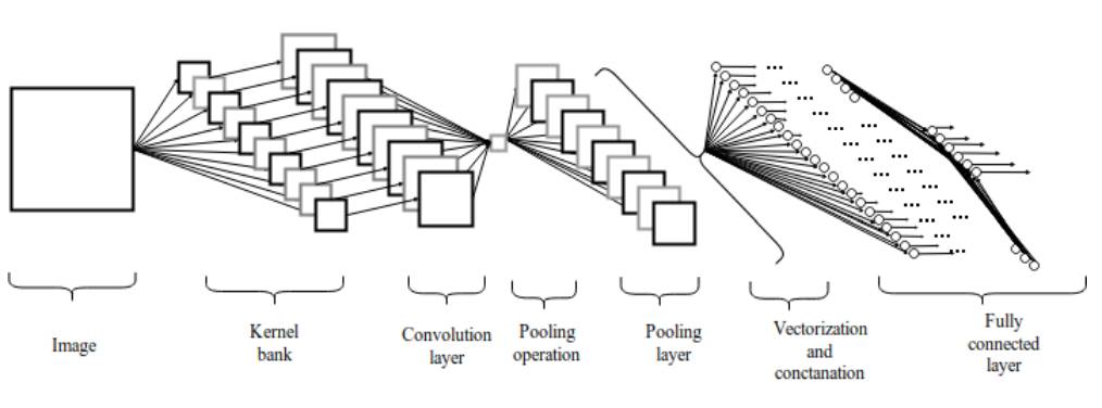
Figure 2.1: Convolutional Neural Network Architecture
2.1 Convolution Layer
The convolution layer consists of a set of parallel feature maps, formed by sliding different convolution kernels over the input image and performing certain operations. Additionally, at each sliding position, an element-wise multiplication and summation operation is performed between the convolution kernel and the input image to project the information within the receptive field onto an element of the feature map. This sliding process can be referred to as stride Z_s, which is a factor controlling the output feature map size. The convolution kernel is much smaller than the input image and acts on the input image either overlapping or in parallel. All elements in a feature map are computed from a single convolution kernel, meaning that one feature map shares the same weights and biases.
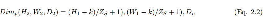
However, using a smaller-sized convolution kernel will lead to imperfect coverage and limit the learning algorithm’s capability. Hence, we generally use zero-padding around the image or the Z_p process to control the size of the input image. Using zero-padding around the image [10] will also control the size of the feature map. During the training process of the algorithm, the dimensions of a group of convolution kernels are generally (k_1, k_2, c), and these convolution kernels slide over a fixed-size input image (H, W, C). Stride and padding are important means of controlling the dimensions of the convolution layer, thus producing feature maps that stack together to form the convolution layer. The size of the convolution layer (feature map) can be calculated using the following formula 2.1.
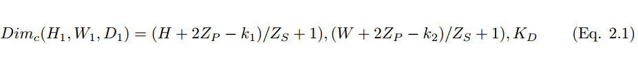
Where H_1, W_1, and D_1 are the height, width, and depth of a feature map, respectively, Z_p is padding, and Z_s is the stride size.
2.2 Activation Function
The activation function defines the output of a neuron given a set of inputs. We pass the weighted sum of linear network input values to the activation function for non-linear transformation. Typical activation functions are based on conditional probabilities, returning 1 or 0 as output values, i.e., op {P(op = 1|ip) or P(op = 0|ip)}. When the network input information ip exceeds a threshold, the activation function returns a value of 1 and passes the information to the next layer; if the network input ip value is below the threshold, it returns a value of 0 and does not pass the information. Based on the separation of relevant and irrelevant information, the activation function determines whether a neuron should be activated. The higher the network input value, the greater the activation. Different types of activation functions have various applications, and some common activation functions are shown in Table 1.
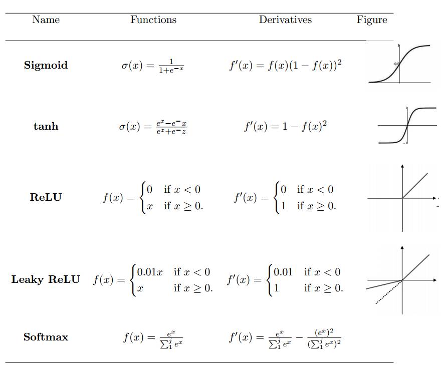
Table 1: Non-linear Activation Functions
2.3 Pooling Layer
The pooling layer refers to the down-sampling layer, which combines the outputs of a cluster of neurons from the previous layer with a single neuron in the next layer. Pooling operations are performed after non-linear activation, where the pooling layer helps reduce the number of parameters and avoid overfitting; it can also serve as a smoothing technique to eliminate unwanted noise. The most common pooling method is simple max pooling, and in some cases, we also use average pooling and L2 norm pooling operations.
When using the number of convolution kernels D_n and stride size Z_s to perform pooling operations, its dimensions can be calculated by the following formula:
2.4 Fully Connected Layer
After the pooling layer, the three-dimensional pixel tensor needs to be converted into a single vector. These vectorized and concatenated data points are then fed into a fully connected layer for classification. The function of the fully connected layer is the weighted sum of features plus bias, which is fed into the activation function’s result. The architecture of the convolution network is shown in Figure 2. This local connection architecture surpasses traditional machine learning algorithms in image classification problems [11] [12].
2.5 Loss or Cost Function
The loss function maps the events of one or more variables to a real number related to a cost. The loss function is used to measure the model’s performance and the inconsistency between the actual values y_i and the predicted values y hat. The model’s performance increases as the value of the loss function decreases.
If the output vector of all possible outputs is y_i = {0, 1} and the event x with a set of input variables x = (xi, x2, …, xt), then the mapping from x to y_i is as follows:
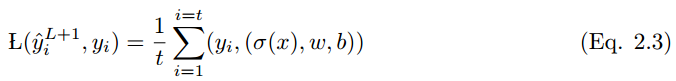
Where L(y_i hat, y_i) is the loss function. Many types of loss functions are applied differently, and some of them are listed below.
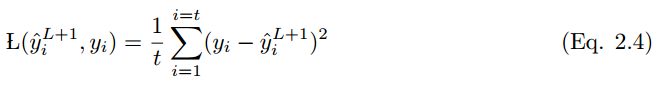
2.5.1 Mean Squared Error
Mean Squared Error (MSE), also known as the squared loss function, is commonly used to evaluate performance in linear regression models. If y_i hat is the output value for t training samples, and y_i is the corresponding label value, then the mean squared error (MSE) is:
The downside of MSE is that when it appears with the Sigmoid activation function, it may lead to slow learning speed (slower convergence).
Other loss functions described in this section include Mean Squared Logarithmic Error, L_2 loss function, L_1 loss function, Mean Absolute Error, and Mean Absolute Percentage Error, etc.
2.5.7 Cross-Entropy
The most commonly used loss function is the cross-entropy loss function, as shown below. If the output y_i has a probability in the training set label  and the probability that output y_i is not in the training set label
 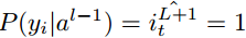 . The expected label is y, thus:
To minimize the cost function,

In the case of i training samples, the cost function is:

3 Learning of Convolutional Networks
3.1 Feedforward Inference Process
The feedforward propagation process of convolutional networks can be mathematically explained as multiplying the input values by randomly initialized weights, then each neuron adds an initial bias term, and finally sums all products of all neurons to feed into the activation function, which performs a non-linear transformation on the input values and outputs the activation results.
In a discrete color space, images and convolution kernels can be represented as three-dimensional tensors of (H, W, C) and (k_1, k_2, c), respectively, where m, n, c represent the pixels at row m and column n of the c-th image channel. The first two parameters represent spatial coordinates, while the third parameter represents the color channel.
If a convolution kernel slides over a color image, the convolution operation of the multi-dimensional tensor can be represented as:
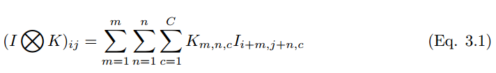
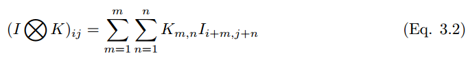
The convolution process can be denoted by the symbol ⓧ. For grayscale scalar images, the convolution process can be represented as,
A convolution kernel  (hereinafter referred to as k_p,q|u,v) slides to the position of image I_m,n with a stride of 1 and with padding. Then the feature map of the convolution layer
  (hereinafter referred to as C_p,q|m,n) can be calculated as
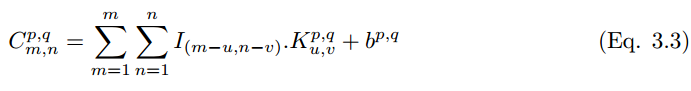
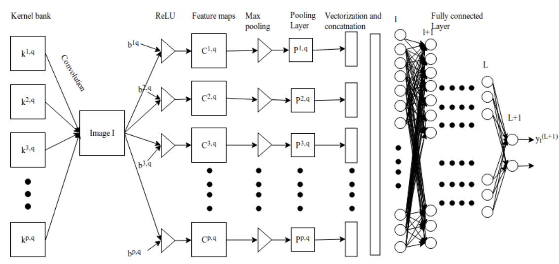
Figure 3.1: Convolutional Neural Network
After performing convolution, we need to use a non-linear activation function to obtain the feature map:
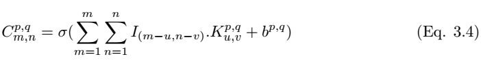
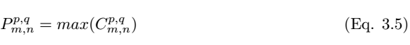
Where σ is the ReLU activation function. The pooling layer P_p,q|m,n can be constructed by selecting the maximum value of m,n from the convolution layer, and the construction of the pooling layer can be written as,
The output of the pooling layer P^p,q can be concatenated into a vector of length p*q, which can then be fed into the fully connected network for classification. The vectorized data points from layer l-1
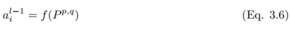
can be calculated using the following equation:
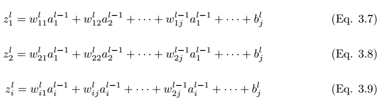
The long vector is fed from layer l to the fully connected network of layer L+1. If there are L fully connected layers and n neurons, then l can represent the first fully connected layer, L represents the last fully connected layer, and L+1 is the classification layer shown in Figure 3.2. The forward propagation process in the fully connected layer can be represented as:
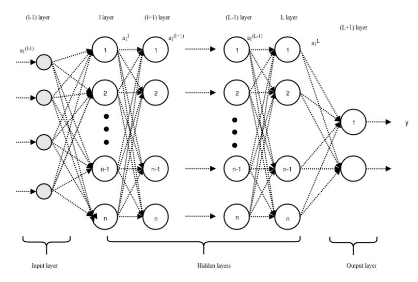
Figure 3.2: Forward Propagation Process in the Fully Connected Layer
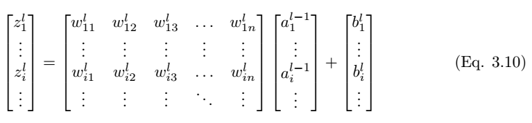
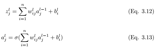
As shown in Figure 3.3, we consider a single neuron (j) in the fully connected layer l. The input values a_l-1,i are weighted by the weights w_ij and added to the bias term b_l,j. Then we feed the input values z_l,i of the last layer into the non-linear activation function σ. The input values of the last layer can be calculated by the following equation,
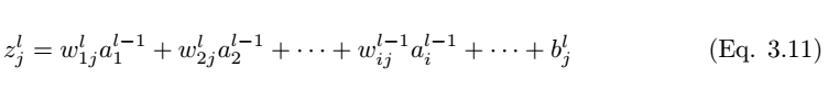
Where z_l,i is the input value of the activation function for neuron j in layer l.
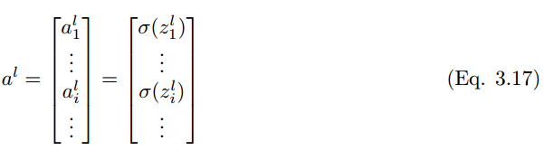
Thus, the output of layer l is
Figure 3.3: Forward Propagation Process of Neuron j in Layer l
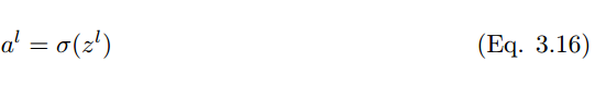
Where a^l is
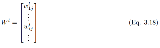
W^l is
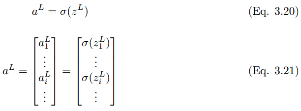
Similarly, the output value of the last layer L is

Where
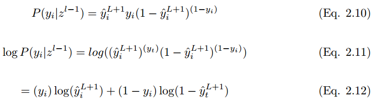
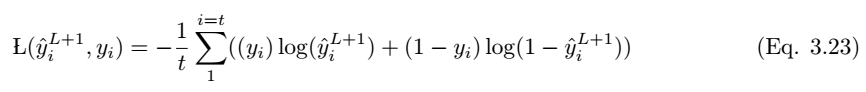
Expanding these to the classification layer, the final output prediction value y_i hat for neuron unit (i) in layer L + 1 can be represented as:

If the predicted value is y_i hat and the actual label value is y_i, then the model’s performance can be calculated using the following loss function equation. According to Eqn.2.14, the cross-entropy loss function is:
This concludes a brief mathematical process of forward propagation. This paper also emphasizes the mathematical process of backward propagation; however, due to space constraints, we do not present it in this article. Interested readers can refer to the original paper.
4 Conclusion
This article provides an overview of the architecture of convolutional neural networks, including different activation functions and loss functions, while detailing the steps of feedforward and backward propagation. For mathematical simplicity, we used grayscale images as input information. The stride value of the convolution kernel is set to 1, with padding applied. The non-linear transformations of the intermediate and final layers are completed using ReLU and sigmoid activation functions. The cross-entropy loss function is used to measure the model’s performance. However, extensive optimization and regularization steps are needed to minimize the loss function, increase the learning rate, and avoid overfitting of the model. This paper attempts to focus solely on the formulation of a typical convolutional neural network architecture with gradient descent optimization.

Click [Read the original text] to register for the competition. For registration in the US division, please click the homepage US to enter the registration channel for the US division.