Build a Neural Network in 100 Lines of Python Code

Produced by Big Data Digest

Source: eisenjulian

Compiled by: Zhou Jiale, Qian Tianpei

Using deep learning libraries like TensorFlow and PyTorch to write a neural network is no longer a novelty.

But do you know how to elegantly build a neural network using Python and NumPy?

Nowadays, there are many deep learning frameworks available, equipped with various important features such as automatic differentiation, graph-based optimization computations, and hardware acceleration. For people, it seems that enjoying the convenience brought by these important features is taken for granted. However, taking a look at what is hidden beneath these features can help you better understand how these networks actually work.

So today, we will guide you step by step to build a neural network. The ingredients are simple Python and NumPy code!

All the code in this article can be found here.

https://colab.research.google.com/github/eisenjulian/slides/blob/master/NN_from_scratch/notebook.ipynb

When computing backpropagation, we can choose to use function symbols and variable symbols to record the differentiation process. They correspond to the edges and nodes in the computation graph.

Given R^n→R and x∈R^n, the gradient is an n-dimensional row vector composed of the partial derivatives ∂f/∂_j(x).

If f:R^n→R^m and x∈R^n, then the Jacobian matrix is an m×n matrix composed of the following functions.

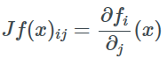
For a given function f and vectors a and b, if a=f(b), we denote the Jacobian matrix as ∂a/∂b, and when a is a real number, it represents the gradient.

Given three vectors a∈A, c∈C from different vector spaces, and two differentiable functions f:A→B and g:B→C such that f(a)=b and g(b)=c, we can obtain the Jacobian matrix of the composite function as the product of the Jacobian matrices of functions f and g:

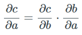
This is the famous chain rule. The backpropagation algorithm, proposed in the 1960s and 1970s, applies the chain rule to calculate the gradient of a real function with respect to its various parameters.

Our ultimate goal is to gradually find the minimum of the function by moving in the opposite direction of the gradient (ideally the global minimum), as doing so will gradually decrease the function value at least locally. When we have two parameters to optimize, the entire process is as shown:

Assuming the function f_i(a_i)=a_i+1 is composed of more than two functions, we can repeatedly apply the formula for differentiation and obtain:

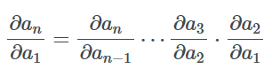
There are many ways to compute this product, the most common being from left to right or from right to left.

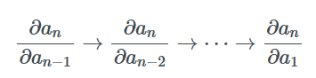
If a_n is a scalar, we can compute the entire gradient by first calculating ∂a_n/∂a_n-1 and then right-multiplying all the Jacobian matrices ∂ai/∂ai_-1. This operation is sometimes referred to as VJP or Vector-Jacobian Product.

Since we start the entire process by calculating ∂a_n/∂a_n-1 and gradually compute ∂a_n/∂a_n-2, ∂a_n/∂a_n-3, etc., while saving intermediate values, this process is called reverse mode differentiation. Ultimately, we can calculate the gradient of a_n with respect to all other variables.

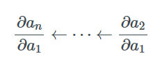
In contrast, the forward mode process is the opposite. It starts by calculating the Jacobian matrix like ∂a₂/∂a₁ and left-multiplying ∂a₃/∂a₂ to compute ∂a₃/∂a₁. If we continue to multiply ∂a_i/∂a_i-1 and save intermediate values, we can ultimately obtain the gradient of all variables with respect to ∂a₂/∂a₁. When ∂a₂/∂a₁ is a scalar, all products are column vectors, which is known as the Jacobian-Vector Product (or JVP).

You might have guessed it; for backpropagation, we prefer to apply the reverse mode—because we want to gradually obtain the gradient of the loss function with respect to each layer’s parameters. Although the forward mode can also compute the required gradients, it is inefficient due to excessive repeated calculations.

The process of calculating gradients may seem like a lot of high-dimensional matrix multiplications, but in reality, the Jacobian matrix is often sparse, block, or diagonal, and since we only care about the result of right-multiplying it by a row vector, we don’t need to waste too much computational and storage resources.

In this article, our method is mainly used for sequentially built neural networks, but the same method also applies to other algorithms or computation graphs that compute gradients.

For a detailed description of reverse and forward modes, you can refer to this link☟

http://colah.github.io/posts/2015-08-Backprop/

In typical supervised machine learning algorithms, we usually utilize a complex function whose input is a tensor containing the numerical features of labeled samples. Additionally, there are many weight tensors used to describe the model.

The loss function is a scalar function concerning samples and weights, which measures the gap between the model output and the expected labels. Our goal is to find the most suitable weights to minimize the loss. In deep learning, the loss function is represented as a composition of a series of simple functions that are easy to differentiate. All these simple functions (except for the final function) are what we refer to as layers, and each layer typically has two sets of parameters: inputs (which can be the outputs of the previous layer) and weights.

The final function represents the loss measurement, which also has two sets of parameters: model output y and true label y^ . For example, if the loss measure l is the squared error, then ∂l/∂y=2 avg(y-y^ ). The gradient of the loss measure will be the initial row vector for applying reverse mode differentiation.

The concept behind automatic differentiation is quite mature. It can be accomplished at runtime or during compilation, but how it is implemented can have a huge impact on performance. I recommend that you carefully read the Python implementation of HIPS autograd to truly understand autograd.

The core idea has actually remained unchanged. From what we learned in school about how to differentiate, we should know this. If we can trace the computations that lead to the final scalar output and we know how to differentiate simple operations (like addition, multiplication, exponentiation, logarithm, etc.), we can calculate the gradient of the output.

Assuming we have a linear intermediate layer f represented by matrix multiplication (ignoring bias for now):

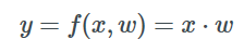
To adjust the w values using gradient descent, we need to compute the gradient ∂l/∂w. Here we can observe that changing y to affect l is key.

Each layer must satisfy the following condition: Given the gradient of the loss function with respect to this layer’s output, we can obtain the gradient of the loss function with respect to this layer’s input (i.e., the output of the previous layer).

Now applying the chain rule twice to obtain the gradient of the loss function with respect to w:

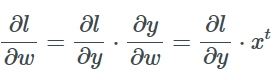
With respect to x:

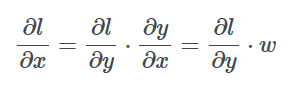
Therefore, we can backpropagate a gradient to update the previous layer and update the inter-layer weights to optimize the loss, and that’s it!

Let’s first take a look at the code or directly try the Colab Notebook.

https://colab.research.google.com/github/eisenjulian/slides/blob/master/NN_from_scratch/notebook.ipynb

We start by encapsulating a class that contains a tensor and its gradient.

Now we can create a layer class, and the key idea is that during forward propagation, we return the output of this layer and a function that can accept output gradients and input gradients, and update the weight gradients in the process.

Then, the training process will have three steps: compute forward pass, then backpropagate, and finally update weights. A key point here is to place the weight update at the end, as weights can be reused across multiple layers, and we prefer to update them only when necessary.

class Layer:  def __init__(self):    self.parameters = []  def forward(self, X):    """    Override me! A simple no-op layer, it passes forward the inputs    """    return X, lambda D: D  def build_param(self, tensor):    """    Creates a parameter from a tensor, and saves a reference for the update step    """    param = Parameter(tensor)    self.parameters.append(param)    return param  def update(self, optimizer):    for param in self.parameters: optimizer.update(param)

The standard practice is to delegate the job of updating parameters to the optimizer, which receives instances of parameters after each batch. The simplest and most well-known optimization method is mini-batch stochastic gradient descent.

class SGDOptimizer():  def __init__(self, lr=0.1):    self.lr = lr  def update(self, param):    param.tensor -= self.lr * param.gradient    param.gradient.fill(0)

Under this framework, and using the results computed earlier, the linear layer is as follows:

class Linear(Layer):  def __init__(self, inputs, outputs):    super().__init__()    tensor = np.random.randn(inputs, outputs) * np.sqrt(1 / inputs)    self.weights = self.build_param(tensor)    self.bias = self.build_param(np.zeros(outputs))  def forward(self, X):    def backward(D):      self.weights.gradient += X.T @ D      self.bias.gradient += D.sum(axis=0)      return D @ self.weights.tensor.T    return X @ self.weights.tensor +  self.bias.tensor, backward

Next, let’s look at another commonly used layer, the activation layer. They belong to pointwise non-linear functions. The Jacobian matrix of a pointwise function is a diagonal matrix, meaning when multiplied by the gradient, it is multiplied pointwise.

class ReLu(Layer):  def forward(self, X):    mask = X > 0    return X * mask, lambda D: D * mask

Calculating the gradient of the Sigmoid function is slightly more challenging, but it is also computed pointwise:

class Sigmoid(Layer):  def forward(self, X):    S = 1 / (1 + np.exp(-X))    def backward(D):      return D * S * (1 - S)    return S, backward

As we build many layers in sequence, we can iterate through them to get the output of each layer in turn. We can store the backward functions in a list and use them during backpropagation to directly obtain the loss gradient with respect to the input layer. It’s that magical:

class Sequential(Layer):  def __init__(self, *layers):    super().__init__()    self.layers = layers    for layer in layers:      self.parameters.extend(layer.parameters)  def forward(self, X):    backprops = []    Y = X    for layer in self.layers:      Y, backprop = layer.forward(Y)      backprops.append(backprop)    def backward(D):      for backprop in reversed(backprops):        D = backprop(D)      return D    return Y, backward

As we mentioned earlier, we will need to define the loss function and gradient for batch samples. A typical example is MSE, which is commonly used in regression problems, and we can implement it like this:

def mse_loss(Yp, Yt):  diff = Yp - Yt  return np.square(diff).mean(), 2 * diff / len(diff)

We are almost there! Now we have defined two types of layers and a method to combine them, how do we train? We can use an API similar to that in scikit-learn or Keras.

class Learner():  def __init__(self, model, loss, optimizer):    self.model = model    self.loss = loss    self.optimizer = optimizer  def fit_batch(self, X, Y):    Y_, backward = self.model.forward(X)    L, D = self.loss(Y_, Y)    backward(D)    self.model.update(self.optimizer)    return L  def fit(self, X, Y, epochs, bs):    losses = []    for epoch in range(epochs):      p = np.random.permutation(len(X))      X, Y = X[p], Y[p]      loss = 0.0      for i in range(0, len(X), bs):        loss += self.fit_batch(X[i:i + bs], Y[i:i + bs])      losses.append(loss)    return losses

That’s it! If you’ve followed my thought process, you may have noticed that there are a few lines of code that can be omitted.

Now we can test our code with some data.

X = np.random.randn(100, 10)w = np.random.randn(10, 1)b = np.random.randn(1)Y = X @ W + B  model = Linear(10, 1)learner = Learner(model, mse_loss, SGDOptimizer(lr=0.05))learner.fit(X, Y, epochs=10, bs=10)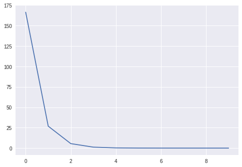

I trained for a total of 10 epochs.

We can also check if the learned weights are consistent with the true weights.

print(np.linalg.norm(m.weights.tensor - W), (m.bias.tensor - B)[0])> 1.848553648022619e-05 5.69305886743976e-06

Alright, it’s that simple. Let’s try a non-linear dataset, such as y=x₁x₂, and add a Sigmoid non-linear layer and another linear layer to make our model a bit more complex, like this:

X = np.random.randn(1000, 2)Y = X[:, 0] * X[:, 1]  losses1 = Learner(    Sequential(Linear(2, 1)),    mse_loss,    SGDOptimizer(lr=0.01)).fit(X, Y, epochs=50, bs=50)  losses2 = Learner(    Sequential(        Linear(2, 10),        Sigmoid(),        Linear(10, 1)    ),    mse_loss,    SGDOptimizer(lr=0.3)).fit(X, Y, epochs=50, bs=50)  plt.plot(losses1)plt.plot(losses2)plt.legend(['1 Layer', '2 Layers'])plt.show()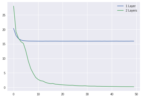

Comparing the training loss of a single layer vs. a two-layer model using the sigmoid activation function.

By building this simple neural network, I hope you have grasped the basic idea of implementing a neural network using Python and NumPy.

In this article, we only defined three types of layers and one loss function, so there is still much to do, but the basic principles are similar. Interested readers can try to implement more complex neural networks!

References

[1] Thinc Deep Learning Library

https://github.com/explosion/thinc

[2] PyTorch Tutorial

https://pytorch.org/tutorials/beginner/nn_tutorial.html[3] Calculus on Computational Graphs

http://colah.github.io/posts/2015-08-Backprop/

[4] HIPS Autograd

https://github.com/HIPS/autograd

Related reports:

https://eisenjulian.github.io/deep-learning-in-100-lines/