-Distilling the Knowledge in a Neural Network

Geoffrey Hinton∗†Google Inc. Mountain View [email protected]

Oriol Vinyals† Google Inc. Mountain View [email protected]

Jeff Dean Google Inc. Mountain[email protected]

Abstract A simple way to improve the performance of almost any machine learning algorithm is to train many different models on the same data and then average their predictions.[3] Unfortunately, making predictions with an ensemble of models can be cumbersome and may be too computationally expensive to deploy to many users, especially if a single model is a large neural network.Caruana and his collaborators[1] have shown that the knowledge in an ensemble of models can be compressed into a single model, making it easier to deploy, and we extend this approach using a different compression technique. We obtained some surprising results on theMNIST dataset, demonstrating that distilling the knowledge of an ensemble into a single model can significantly improve the acoustic model of a widely used commercial system. We also introduce a new type of ensemble consisting of one or more full models and many expert models that learn to distinguish fine-grained categories that are confused by the full model. Unlike expert mixtures, these expert models can be trained quickly in parallel.

Table of Contents

1Introduction

2Distillation

3Preliminary Experiments on MNIST

4Speech Recognition Experiments

4.1Results

5Training Expert Ensembles on Very Large Datasets

5.1JFT Dataset

5.2Expert Models

5.3Assigning Expert Categories

5.4Expert Ensemble for Inference

5.5Results

6Soft Targets as Regularizers

7Relevance of Expert Mixture Models

8Discussion

Many insects have a juvenile form that extracts energy and nutrients from the environment and a completely different adult form that is specialized for travel and reproduction..

In large-scale machine learning, although the requirements for training and deployment phases are completely different, we typically use very similar models: for tasks like speech and object recognition, the training phase must extract structure from very large, highly redundant datasets, which does not require real-time operation and can use a lot of computational resources. However, in the case of deployment to a large number of users, the response time and computational resource requirements are much stricter.The insect analogy suggests that if it makes it easier to extract structure from data, we should be willing to train very cumbersome models. Such cumbersome models can be an ensemble of models trained separately or a very large model trained with very strong regularization methods (such asdropout). Once the cumbersome model is trained, we can use a different type of training called“distillation” to transfer knowledge from the cumbersome model to a smaller model that is more suitable for deployment. A version of this strategy has already been pioneered byRich Caruana and his collaborators. In their important paper, they convincingly showed that the knowledge gained from a large number of models can be transferred to a single small model.

A conceptual barrier that might prevent further investigation of this very promising method is that we tend to equate the knowledge in trained models with learned parameter values, making it difficult to see how to change the form of the model while retaining the same knowledge. A more abstract view of knowledge, freeing it from any specific instantiation, is that it is a learned.

Mapping input vectors to output vectors. For cumbersome models that learn to distinguish a large number of categories, the conventional training objective is to maximize the average log probability of the correct answer, but the side effect of learning is that the trained model assigns probabilities to all incorrect answers, even if these probabilities are very small, some of which are much larger than others. The relative probabilities of incorrect answers tell us important information about how the cumbersome model tends to generalize. For example, an image of a BMW car might be misclassified as a garbage truck with a very small probability, but that error is still much more likely than misclassifying it as a carrot.

It is generally considered that the objective function used for training should reflect the true goals of the user as closely as possible. Nevertheless, models are often trained to optimize performance on the training data, while the true goal is to generalize well to new data. Clearly, it is best to train models to generalize well, but this requires information about how to generalize correctly, which is often not available. However, when we distill knowledge from a large model into a small model, we can train the small model to generalize in the same way as the large model. If the cumbersome model generalizes well, for example, if it is an average of several different models, then the small model trained to generalize in the same way usually performs better on test data than a small model trained in the normal way on the same training set.

One obvious way to transfer the generalization ability of a cumbersome model to a small model is to use the class probabilities produced by the cumbersome model as training“soft targets”. For this transfer phase, we can use the same training set or a separate“transfer” set. When the cumbersome model is a large ensemble composed of a set of simple models, we can use the arithmetic or geometric mean of their respective predicted distributions as soft targets. When soft targets have high entropy, they provide much more information in each training case than hard targets, and the gradient changes between training cases are much smaller, so the small model can often be trained on much less data than the original cumbersome model and using a higher learning rate.

For tasks likeMNIST where cumbersome models almost always produce correct answers with very high confidence, most of the information about the learning function exists in the very small probability ratios of the soft targets. For example, for a version of the digit2, the probability of being classified as the digit3 might be10^-6, and the probability of being classified as the digit7 might be10^-9, while for another version, it might be just the opposite. This is valuable information that defines rich similar structures in the data (i.e., telling us which digit2 looks like digit3, which looks like digit7), but during the transfer phase, the influence on the cross-entropy loss function is very small because the probabilities are close to zero.Caruana and his collaborators circumvented this problem by usinglogits (the inputs to the final softmax function) instead of the probabilities generated by the softmax function as the targets for learning the small model, and minimizing the squared difference between the logits produced by the cumbersome model and those produced by the small model. Our more general solution, called“distillation“, is to raise the temperature of the final softmax function until the cumbersome model produces a set of suitable soft targets. Then, during the training of the small model, we use the same high temperature to match these soft targets. We will later show that matching the logits of the cumbersome model is actually a special case of distillation.

The transfer set used for training the small model can consist entirely of unlabeled data[1] or can use the original training set. We find that using the original training set works well, especially if we add a small term in the objective function that encourages the small model to predict the true target and match the soft targets provided by the cumbersome model. Typically, the small model cannot match the soft targets perfectly, and making incorrect progress towards the correct answer is found to be helpful.

2 Distillation

Neural networks typically produce class probabilities using a“softmax” output layer that converts the logitszi for each class into probabilitiesqi, by comparingzi to the other logits.

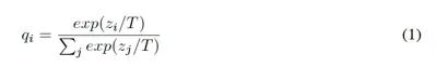
T is a temperature that is usually set to1. Using a higher value produces a softer class probability distribution.

In the simplest form of distillation, knowledge is passed to the distillation model by training it on a transfer set and using the soft target distribution generated at high temperature by thesoftmax function for each case in the transfer set. During the training of the distillation model, the same high temperature is used, but after training is complete, the distillation model uses a temperature of1.

When the correct labels for all or part of the transfer set are known, significant improvements can be made by training the distilled model to produce the correct labels. One approach is to modify the soft targets using the correct labels, but we find that a better approach is to simply use a weighted average of two different objective functions. The first objective function is the cross-entropy with the soft targets, which is computed using the same temperature in the softmax as when generating the soft targets from the cumbersome model. The second objective function is the cross-entropy with the correct labels, which is computed using the same logits in the distilled model but with a temperature of1. We find that the best results are typically obtained by using a lower weight on the second objective function. Since the size of the gradient produced by the soft targets is scaled by1/T^2, it is important to multiply them byT^2 when using both hard and soft targets at the same time. This ensures that if the temperature of distillation is changed while tuning meta-parameters, the relative contributions of hard and soft targets remain approximately constant.

2.1 Matchinglogits is a special case of distillation

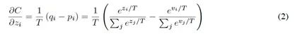
Each case in the transfer set contributes a cross-entropy gradientdC/dzi to the logits of the distillation model. If the cumbersome model produces soft target probabilitiespi from logitsvi, and the transfer training is done at temperatureT, then the gradient is given by:

If the temperature is high relative to the magnitude of the logits, we can approximate:

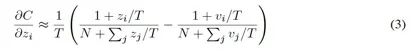
If we now assume that the logits have been zero-centered for each transfer case so thatj zj = Pj vj = 0, then equation3 simplifies to:

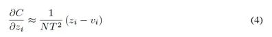
In the high-temperature limit, distillation is equivalent to minimizing1/2(zi −vi)2, provided that the logits for each transfer case are zero-centered. At lower temperatures, the distillation focuses much less on matching the lower logits. This can be beneficial since these logits are almost completely uncorrelated with the cost function used to train the cumbersome model and can be very noisy. On the other hand, these very low logits may convey useful information that the cumbersome model has learned. Which effect dominates is an empirical question. We show that when the distilled model is too small to capture all the knowledge in the cumbersome model, an intermediate temperature works best, strongly suggesting that ignoring the larger negative logits may be helpful.

3 Preliminary Experiments on MNIST

To see how distillation works, we trained a separate large neural network with two hidden layers, each containing1200 rectified linear hidden units, on all60,000 training cases. The network was strongly regularized usingdropout and weight constraints as described in[5]. Dropout can be seen as a method of training an ensemble of models with shared weights. Additionally, the input images were jittered by up to two pixels in any direction. The network achieved67 test errors, while a smaller network with two hidden layers, each containing800 rectified linear hidden units without regularization achieved146 errors. But if this smaller network was regularized by adding an additional task to match the soft targets produced by the large network at a temperature of20, it achieved74 test errors. This suggests that soft targets can transfer a lot of knowledge to the distilled model, including generalization knowledge learned from the training data, even though the transfer set contains no examples of that translation.

When the distilled network has300 units or more in each of its two hidden layers, all results obtained with temperatures greater than8 are quite similar. However, when this is reduced to each layer having30 units, temperatures in the range of2.5 to4 perform significantly better.

We then tried omitting all examples of the digit3 from the transfer set. Thus, from the perspective of the distilled model,3 is a digit it has never seen. Nevertheless, the distilled model only produced206 errors on the test set, of which133 were on the1010 examples of the digit3 in the test set. Most errors were due to learning bias against the3 class being too low. If we increase this bias to3.5 (which optimizes overall performance on the test set), the distilled model produces109 errors, of which14 are on the digit3. Thus, with the correct bias, despite never seeing the digit3 during training, the distilled model correctly identifies98.6% of the test digits3. If the transfer set only contains examples of digits7 and8, then the distilled model produces47.3% test errors, but when the bias for7 and8 is reduced to7.6 to optimize test performance, this number drops to13.2% test errors.

4 Speech Recognition Experiments

In this section, we investigate the impact of ensembles for deep neural network (DNN) acoustic models in automatic speech recognition (ASR). We show that the distillation strategy we propose in this paper achieves the expected effect of distilling a set of models into a single model that performs significantly better than a model of the same size learned directly from the same training data.

Currently, state-of-the-art automatic speech recognition (ASR) systems use deep neural networks (DNN) to map (short-term) temporal context features extracted from waveforms to the probability distributions of discrete states of hidden Markov models (HMM)[4]. Specifically, theDNN produces a probability distribution over a tri-phone state group at each time point, and then the decoder finds a path through theHMM states that balances the use of high-probability states with generating transcriptions that conform to the language model.

Although it is possible (and desirable) to train theDNN to consider the decoder (and the language model) by marginalizing over all possible paths, it is usually trained to perform frame-by-frame classification by minimizing the cross-entropy between the predictions made by the network and the ground truth sequence of states for each observation, given the labels:

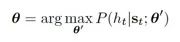
θ is the parameters of our acoustic modelP mapping the acoustic observationst at timet to a probabilityP(ht|st;θ′) of the“correct” HMM stateht, which is determined by the forced alignment with the correct word sequence. The model is trained using distributed stochastic gradient descent.

We adopted an architecture with8 hidden layers, each containing2560 rectified linear units, and a finalsoftmax layer with14,000 labels (HMM targetsht). The input consists of26 frames of40 Mel-scaled filter bank coefficients, with a frame interval of10 milliseconds, and we predict the21th frame’sHMM state. The total number of parameters is about85M. This is a slightly older version of the acoustic model used for Android voice search and should be seen as a very strong baseline. To train theDNN acoustic model, we used about2000 hours of English speech data, producing about700M training samples. The system achieved58.9% frame accuracy and10.9% word error rate (WER).

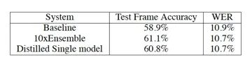
Table1: Classification accuracy andWER show that the performance of the distilled single model is comparable to the average predictions of10 models used to create the soft targets.

4.1 Results

We trained10 separate models to predictP(ht|st;θ), using exactly the same architecture and training procedure as the baseline. These models were randomly initialized with different initial parameter values, and we found that this produced enough diversity in the trained models such that the average predictions of the ensemble model could significantly outperform individual models. We tried to increase diversity among the models by varying the datasets seen by each model, but we found this did not significantly change our results, so we opted for the simpler approach. For distillation, we experimented with temperatures of[1,2,5,10], and used a relative weight of0.5 on the cross-entropy with hard targets, where the bold indicates the best value used in Table1.

Table1 shows that our distillation method can extract more useful information from the training set than simply training a single model with hard labels. The ensemble model of10 models achieved over80% improvement in frame classification accuracy, which translates to a similar improvement observed in distilled models in our preliminary experiments onMNIST. Due to the mismatch in objective functions, the ensemble model had a smaller final target improvement onWER on the23K word test set, but similarly, the ensemble model’s improvement onWER also translated to the distilled model.

Recently, we learned of related work that learns a small acoustic model by matching the class probabilities of a large trained model[8]. However, they distilled using a large-scale unlabeled dataset at a temperature of1, and their best distilled model only reduced the error rate of the small model by28%, which is the percentage difference between the error rates of the large model and the small model when trained with hard labels.

5 Training Expert Ensembles on Very Large Datasets

Training a model ensemble is a very simple way to leverage parallel computation, the usual objection is that the model ensemble requires too much computation at test time, which can be solved by using distillation. However, there is another important objection to model ensembles: if individual models are large neural networks, and the dataset is very large, then the computation required during training is excessive, even though it is easy to parallelize.

In this section, we provide an example of such a dataset and show how to learn expert models, each focusing on a different subset of confusable categories, which can reduce the total computation required for learning the ensemble.

The main problem with experts that focus on making fine-grained distinctions is that they are prone to overfitting, and we will introduce how to use soft targets to prevent overfitting.

5.1 JFT Dataset

JFT is an internal dataset atGoogle containing100 million labeled images with15,000 labels. At the time we conducted this work,Google‘s benchmark model forJFT was a deep convolutional neural network trained for about six months using a large number of cores with asynchronous stochastic gradient descent. This training used two types of parallel processing.

First, many copies of the neural network run on different sets of cores, processing different mini-batch data from the training set. Each copy computes the average gradient of its current mini-batch data and sends that gradient to a sharded parameter server, which sends back new values of the parameters. These new values reflect all gradients received by the parameter server since the last time it sent parameters to the copies. Second, each copy is distributed over multiple cores by placing different subsets of neurons on each core. Ensemble training is another type of parallel processing that can be achieved.

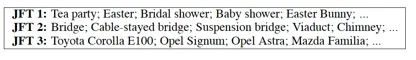
Table2: Example categories derived from our covariance matrix clustering algorithm.

It can only run better relative to the other two types when more cores are available. Waiting years to train a set of models is not feasible, so we need a faster way to improve the baseline model.

5.2 Expert Models

When the number of classes is very large, it makes sense to turn a cumbersome model into an ensemble model that contains a general model trained on all data and many“expert” models, each trained on data rich in examples from a subset of easily confused categories (e.g., different types of mushrooms). Thesoftmax of this type of expert can become smaller by merging all categories it does not care about into a garbage category.

To reduce overfitting and share the work of learning lower-level feature detectors, each expert model is initialized with the weights of the general model. Then, by training the expert model, these weights are slightly modified, with half of the examples coming from its specific subset and the other half randomly sampled from the rest of the training set. After training, we can correct the bias towards the training set by increasing the logit of the garbage category relative to the oversampling of the expert category.

5.3Assigning Expert Categories

To derive the grouping of object categories for the experts, we decided to focus on the categories that our ensemble model often confuses. While we could calculate the confusion matrix and use it as one way to look up these clusters, we chose a simpler method that does not require true labels to build these clusters.

Specifically, we applied a clustering algorithm to the covariance matrix of the predictions of our ensemble model, so that a set of categories that often predict togetherSm will be used as the target for one of our expert modelsm. We applied an online version of theK-means algorithm to the columns of the covariance matrix and obtained reasonable clustering results (as shown in Table2).

5.4 Expert Ensemble for Inference

Before investigating the distillation of expert models, we wanted to see how the ensemble model containing experts performs. In addition to the expert models, we always have a general model to handle categories for which we have no experts and decide which expert models to use. Given an input imagex, we performtop-one classification in two steps.

Step1: For each test case, we find the topn categories with the highest probability according to the general model. Let this set of categories be calledk. In our experiments, we usedn = 1.

Step2: We then take all expert modelsm whose special subset of confusable classesSm has a non-empty intersection withk and call this the active set of expertsAk (note that this set may be empty). We then find the probability distributions of all classesq that minimize:

KL representsKL divergence, whilepm andpg represent the probability distributions of the expert model or full model. Thepm is the distribution overm expert classes and one garbage class, so when calculating its KL divergence with the globalq distribution, we sum the probabilities of all categories in the garbage ofm.

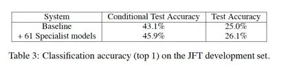
Table3: Classification accuracy on the JFT development set (Top 1).

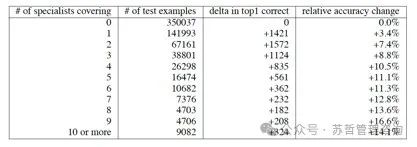
Table4: On the JFT test set, the number of expert models covering the correct category and the increase inTop 1 accuracy.

The equation5 does not have a universal closed-form solution, although when all models produce a probability for each category, the solution is either the arithmetic mean or the geometric mean, depending on whether we useKL(p,q) orKL(q,p). We parameterizeq = softmax(z) (whereT = 1), and optimize the logitsz with gradient descent with respect to equation5. Note that this optimization must be performed for each image.

5.5 Results

Starting from the trained benchmark full network, the experts train very quickly (in days rather than weeks forJFT). Additionally, all experts are trained completely independently. Table3 shows the absolute test accuracy of the benchmark system and the benchmark system combined with expert models. Using61 expert models, the overall test accuracy improved by4.4%. We also report the conditional test accuracy, which is the accuracy considering only the examples belonging to the expert category, limiting our predictions to that subset of categories.

For our JFT expert experiments, we trained61 expert models, each with300 classes (plus a trash class). Since the category sets of experts are not disjoint, we often have multiple experts covering a specific image category. Table4 shows the number of test set samples, the number of samples correctly classified at the first position when using experts, and the relative percentage increase intop1 accuracy for the JFT dataset, broken down by the number of experts covering that category. We are encouraged by this overall trend that when we have more experts covering a specific category, the accuracy improvement is greater, as training independent expert models is very easy to parallelize.

6 Soft Targets as Regularizers

One of the main points of using soft targets instead of hard targets is that soft targets can carry a lot of useful information that cannot be encoded by a single hard target. In this section, we demonstrate this effect significantly by fitting the baseline speech model described earlier with85M parameters using less data. Table5 shows that training the baseline model using only3% of the data (about20M examples) with hard targets leads to severe overfitting (we did early stopping because the accuracy dropped sharply after reaching44.5%), while the same model trained with soft targets can recover almost all the information from the full training set (just under2%). More importantly, we do not need to do early stopping: the system with soft targets simply“converges” to57%. This indicates that soft targets are a very effective way to convey the patterns discovered by a model trained on the full data to another model.

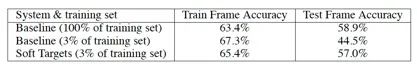
Table5: Soft targets allow a new model to generalize well even when using only3% of the training set. These soft targets are obtained by training on the full training set.

Using soft targets to prevent overfitting in experts.

In our experiments using the JFT dataset, the experts categorized all their non-expert classes into a garbage category. If we allow experts to perform a full softmax operation over all categories, there may be a better way to prevent them from overfitting than using early stopping strategies. Experts are trained on data that is highly enriched in their expert categories. This means that the effective size of their training sets is much smaller, and they have a strong tendency to overfit to their expert categories. It is not feasible to solve this problem by reducing the size of the experts, as this would lose the very helpful transfer effects gained from modeling all non-expert categories.

Our experiments using3% of the speech data strongly suggest that if an expert’s weights are set to those of the general model, we can retain almost all knowledge about non-expert categories by training on soft targets for those non-expert categories, rather than using hard targets. Soft targets can be provided by the general model. We are currently exploring this approach.

7 Relevance of Expert Mixture Models

The use of expert teams, which are trained on subsets of data, has some similarities to expert mixture models[6] that use gating networks to compute the probabilities of assigning each example to each expert. While the experts learn to handle examples assigned to them, the gating network is learning to choose which expert to assign each example based on the relative discriminative performance of the experts on that example. Leveraging the discriminative performance of the experts to determine how to allocate learning is much better than simply clustering the input vectors and assigning one expert to each cluster, but it makes training difficult to parallelize: first, the weighted training set for each expert continually changes in a way that depends on all other experts, and second, the gating network needs to compare the performance of different experts on the same example to understand how to modify its allocation probabilities. These difficulties mean that expert mixture models are rarely used in areas where they might be most beneficial: tasks on large datasets containing clearly distinct subsets.

It is much easier to parallelize the training of multiple expert models. We first train a general model, then use the confusion matrix to define the subsets for expert training. Once these subsets are defined, the experts can be trained completely independently. At test time, we can use the predictions of the general model to decide which experts are relevant, and only those experts need to run.

8 Discussion

We have demonstrated that distillation is very effective for transferring knowledge from an overall model or a large, highly regularized model to a smaller, distilled model. In theMNIST dataset, even when examples of one or more categories are missing from the transfer set used to train the distilled model, distillation is still very effective. For a deep acoustic model, which is a version used for Android voice search, we have shown that nearly all improvements achieved by training a deep neural network ensemble can be distilled into a single neural network of the same size that is easier to deploy.

For very large neural networks, even training a complete ensemble model is not feasible, but we have shown that the performance of a single large network trained for a very long time can be significantly improved by learning a large number of expert networks, each of which learns to distinguish highly confusable categories. We have not yet shown that we can distill the knowledge of the experts back into a single large network.

Thanks

We thankYangqing Jia for assisting in training the models onImageNet, andIlya Sutskever andYoram Singer for helpful discussions.

References

1.C. Buciluaˇ, R. Caruana andA. Niculescu-Mizil. Model compression. In Proceedings of the 12th ACM SIGKDD International Conference on Knowledge Discovery and Data Mining,KDD’06, 535-541, 2006. New York, USA. ACM.

2.J. Dean, G. S. Corrado, R. Monga, K. Chen, M. Devin, Q. V. Le, M. Z. Mao, M. Ranzato, A. Senior, P. Tucker, K. Yang, and A. Y. Ng. Large scale distributed deep networks. In NIPS, 2012. Large scale distributed deep networks. InNIPS,2012.

3.T. G. Dietterich. Ensemble methods in machine learning.. In Multiple classifier systems,, pages 1-15. Springer, 2000.

4.G. E. Hinton, L. Deng, D. Yu, G. E. Dahl, A. Mohamed, N. Jaitly, A. Senior, V. Vanhoucke, P. Nguyen, T. N Sainath, and B. Kingsbury. Deep neural networks for acoustic modeling in speech recognition: The shared view of four research teams.IEEE Signal Processing Magazine,29(6):82–97,2012.

5.G. E. Hinton, N. Srivastava, A. Krizhevsky, I. Sutskever, and R. R. Salakhutdinov. Improving neural networks by preventing co-adaptation of feature detectors. arXiv preprint arXiv:1207.0580, 2012.

6.R. A. Jacobs, M. I. Jordan, S. J. Nowlan, and G. E. Hinton. Adaptive mixtures of local experts. Neural Computation,3(1):79-87,1991.

7.Krizhevsky, I. Sutskever, and G. E. Hinton. Imagenet classification with deep convolutional neural networks. In Advances in Neural Information Processing Systems, pages 1097–1105, 2012. –In Chinese:Krizhevsky, I. Sutskever andG. E. Hinton. Using deep convolutional neural networks forImagenet classification. InAdvances in Neural Information Processing Systems, pages 1097–1105, 2012.

8.J. Li, R. Zhao, J. Huang, and Y. Gong. A small DNN learning method based on output distribution criterion.. In Proceedings of the 2014 Interspeech Conference, pages 1910-1914, 2014.

9.N. Srivastava, G.E. Hinton, A. Krizhevsky, I. Sutskever, and R. R. Salakhutdinov. Dropout: A simple way to prevent neural networks from overfitting. The Journal of Machine Learning Research, 15(1):1929–1958,2014. N. Srivastava, G.E. Hinton, A. Krizhevsky, I. Sutskever, andR. R. Salakhutdinov. Dropout: A simple method for preventing neural networks from overfitting.Machine Learning Research Journal, 15(1):1929–1958,2014.