Currently, there are applications based on Transformer in three major image problems:Classification (ViT), Detection (DETR) and Segmentation (SETR), all achieving good results. In the future, could Transformer possibly replace CNN? Will Transformer revolutionize the CV field just like its application in NLP? What might the research directions be? Please look forward to the next article for answers.
01
Concepts and Framework
Transformer is a milestone model proposed by Google in 2017, and it is also a key technology in the language AI revolution. Prior to this, the SOTA models were all based on recurrent neural networks (RNNs, LSTMs, etc.). Essentially, RNNs process data in a serial manner, which corresponds to NLP tasks, meaning each word is processed one at a time in the order they appear in the sentence.
In contrast to this serial approach, the significant innovation of Transformer lies in parallelized language processing: all words in the text can be analyzed simultaneously rather than in sequential order. To support this parallel processing, Transformer relies on the attention mechanism. The attention mechanism allows the model to consider the relationship between any two words, regardless of their position in the text sequence. By analyzing the pairwise relationships between words, it determines which words or phrases should receive more attention.
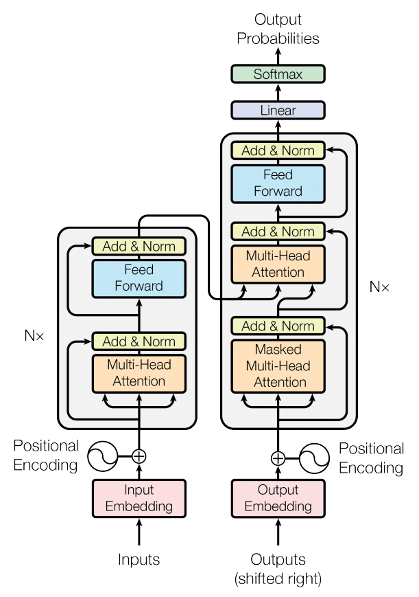
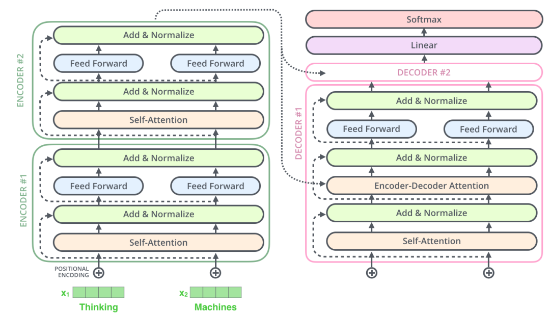
Transformer adopts an Encoder-Decoder architecture, and the diagram below illustrates the structure of Transformer. The left half represents the encoder, while the right half represents the decoder [1]:
Various existing models based on Transformer are primarily related to NLP tasks. However, some recent articles have innovatively applied Transformer models across domains to computer vision tasks, achieving impressive results. This is considered by many AI scholars to herald a new era in the CV field, potentially completely replacing traditional convolution operations.
Recently, many articles in the CV field have transferred transformers, which can generally be categorized into two major types:
-
Combining self-attention mechanisms with common CNN architectures
-
Completely replacing CNN with self-attention mechanisms
Among them, the paper under review at ICLR 2021 titled “An Image Is Worth 16X16 Words: Transformers for Image Recognition at Scale” [2] adopts the second approach.
02
Implementation Details
2.1 Encoder
The Encoder layer consists of six identical layer structures, each containing two sub-layers. The first sub-layer is the Multi-Head Attention Layer (orange part), and the second sub-layer is the Feed Forward Layer (light blue part). Additionally, there is a residual connection that directly passes the input embedding to the first Add & Norm layer (yellow part) and from the first Add & Norm layer to the second Add & Norm layer (i.e., the pink-yellow 1 and yellow 1-yellow 2 parts in the diagram utilize the residual connection).
2.2 Decoder
The Decoder layer also consists of six identical layer structures, but it is slightly more complex than the Encoder layer. It has three sub-layer structures: the first sub-layer is the Masked Multi-Head Attention Layer (orange part), the second sub-layer is the Multi-Head Attention Structure (orange part), and the third sub-layer is the Feed Forward Layer (light blue part).
Notes:
-
The residual connections in this part are the pink-yellow 1, yellow 1-yellow 2, and yellow 2-yellow 3 sections.
-
The focus of this layer is the second sub-layer, which is the multi-head attention layer. Its input includes two parts: the output of the first sub-layer and the output of the Encoder layer (this is one of the distinctions from the encoder layer), thus linking the encoder and decoder layers for information exchange between words, where this information exchange is achieved through shared weights WQ, WV, WK.
-
The mask in the first sub-layer serves to prevent the use of future output words during training. For instance, during training, the first word cannot refer to the generation result of the second word, thus the second word and all subsequent words are masked. In general, the mask ensures that the information at position i can only be based on outputs smaller than i.
-
Residual structures are used to address the vanishing gradient problem and can increase the complexity of the model.
-
The LayerNorm layer is used to normalize the output of the attention layer, transforming it into a normal distribution with a mean of 0 and a variance of 1. In CV, batchNorm is often used, which normalizes the samples within a batch size, while layernorm normalizes across a layer. The two serve the same purpose but target different dimensions; generally, the input dimension is (batch_size, seq_len, embedding), where batchnorm processes the batch_size layer, while layernorm processes seq_len (i.e., batchnorm normalizes across a batch of samples, while layernorm normalizes each sample).
-
The reason for using ln instead of bn is due to the varying lengths of input sequences. Each sequence has a different length; although padding is applied, the padding zeros are actually useless information, and the useful information still resides in the sequence information. Since the lengths of sequences differ, bn cannot be uniformly applied here.
-
FFN consists of two fully connected layers: w * [delta(w * x + b)] + b, where delta is the ReLU activation function. The reason for using the FFN layer is to utilize a non-linear function to fit the data. If the aim is merely non-linear fitting, the first layer suffices; however, the reason for using two fully connected layers is that the output dimension of the first layer is (batch_size, seq_len, dff) (where dff is a hyperparameter set to 2048), and the second fully connected layer is used to transform dff back to the initial d_model (512) dimension.
-
The input to the multi-head self-attention mechanism in the decoder layer consists of two parameters—the output of the encoder layer and the output of the first layer of the masked multi-head self-attention mechanism in the decoder layer, where q=encoder’s output, k=v=decoder’s output.
-
The input to the encoder contains two parts: a sequence of token embeddings + positional embeddings, calculated using sine and cosine functions for the positions in the sequence (even positions use sine, odd positions use cosine).
2.3 Self-Attention
Self-Attention is a method used by Transformer to find and focus on words relevant to the current word. For example:
The animal didn’t cross the street because it was too tired.
Here, it is unclear whether it refers to animal or street, which is difficult for the algorithm to determine, but self-attention can link it to animal, achieving disambiguation.
The specific process of self-attention is illustrated in the diagram below:
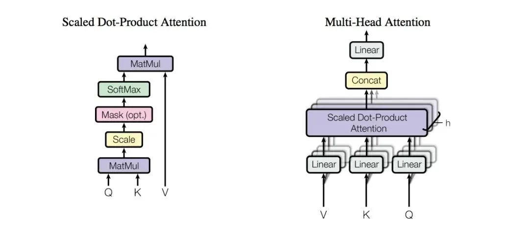
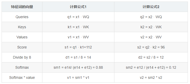
As shown in the diagram, the attention mechanism primarily involves three vectors Q(Query), K(Key), V(Value), and the computation process of these three vectors is illustrated in the diagram below:
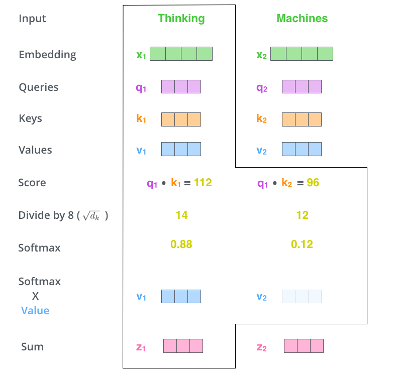
In the diagram, WQ, WV, WK are three randomly initialized matrices, and the computation formula for each feature word’s vector is as follows:
Notes:
-
Score indicates the relevance of the attended word.
-
This method of determining the weight distribution of value based on the similarity between query and key is called scaled dot-product attention.
-
Difference between attention and self-attention:
-
Self-attention is a special case of general attention, where in self-attention, Q=K=V, and each unit in the sequence computes attention with all units in that sequence. The multi-head attention proposed by Google captures relevant information across different sub-controls by computing multiple times.
-
The characteristic of self-attention is that it ignores the distance between words and directly computes dependencies, allowing it to learn the internal structure of a sentence, making it relatively simple and enabling parallel computation. Some papers have suggested that self-attention can be treated as a layer and used in conjunction with RNN, CNN, FNN, etc., successfully applied to other NLP tasks.
-
The reason for dividing the attention by 8 (sqrt(d_k)) is for scaling, which disperses attention; original attention values concentrate on the highest score, achieving a weight of 1; after scaling, the attention values are more dispersed.
-
The reason for dividing by sqrt(d_k) is that the original representation x1 follows a normal distribution with a mean of 0 and a variance of 1, and after multiplying by the weight matrix, the result follows a normal distribution with a mean of 0 and a variance of d_k, so to avoid altering the original representation’s distribution, it must be divided by sqrt(d_k).
Advantages of the Attention Mechanism:
-
It captures global and local relationships in one step, not constrained by the sequence length limitations that RNNs face in capturing long-term dependencies.
-
The result of each step does not depend on the previous step, allowing for a parallel processing mode.
-
Compared to CNN and RNN, it has fewer parameters and lower model complexity.
Disadvantages of the Attention Mechanism:
It cannot capture positional information, meaning it cannot learn the order relationships in the sequence. This can be improved by adding positional information, such as through position vectors, as seen in the BERT model.
2.4 Multi-Headed Attention
The multi-headed attention mechanism involves multiple sets of Q, K, V matrices, with each set representing one computation of the attention mechanism. The transformer uses 8 sets, resulting in 8 matrices, which are concatenated and then multiplied by a parameter matrix WO to yield the final output of the multi-attention layer. The entire process is illustrated in the diagram below:

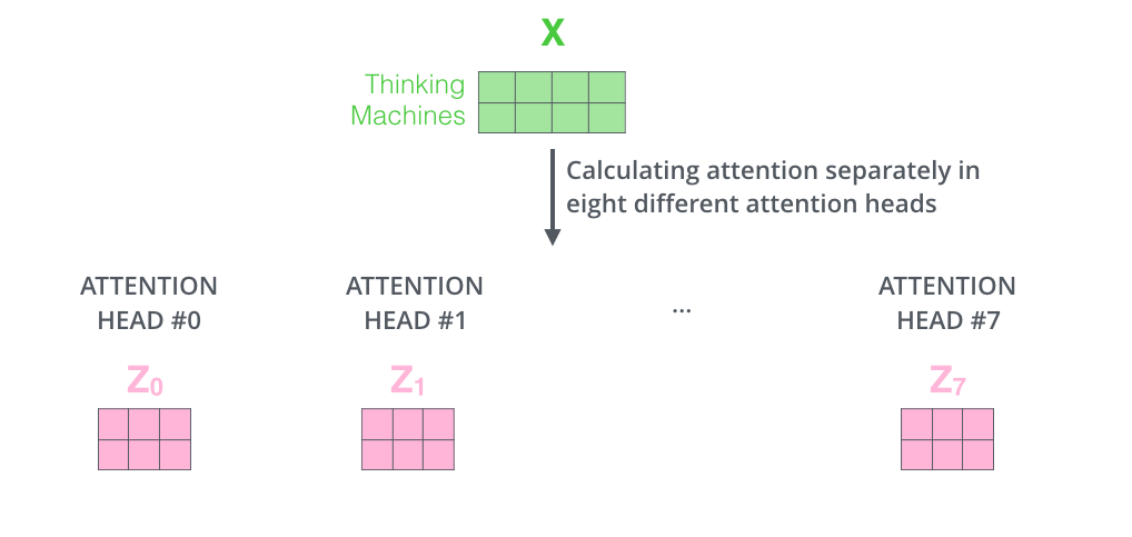
The left diagram shows the use of multiple sets of Q, K, V matrices, while the right diagram shows that calculating with 8 sets of Q, K, V matrices yields 8 matrices, which must be computed and output as one matrix to serve as the final output of the multi-attention layer. As shown in the diagram, WO is a randomly initialized parameter matrix.
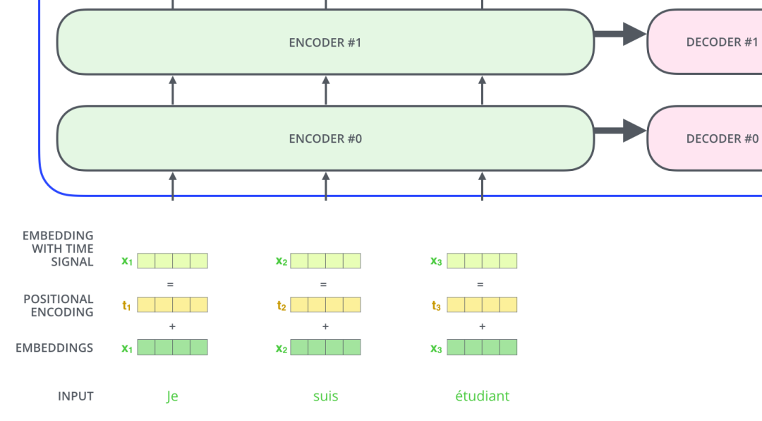
2.5 Positional Encoding
In the figure, there is also a vector positional encoding, which exists to explain the order of words in the input sequence, with dimensions consistent with the embedding dimensions. This vector determines the position of the current word, or the distance between different words in a sentence. The calculation method in the paper is as follows:
PE(pos,2 * i) = sin(pos / 10000^{2i/d_{model}}) PE(pos,2 * i + 1) = cos(pos / 10000^{2i/d_{model}})
Where pos refers to the current word’s position in the sentence, and i refers to the index of each value in the vector. From the formula, it can be seen that even-positioned words in the sentence use sine encoding, while odd-positioned words use cosine encoding. Finally, the values of positional encoding are added to the embedding values as input to the transformer structure, as shown in the diagram below:
2.6 Layer Normalization
In the transformer, each sub-layer (self-attention layer, fully connected layer) is followed by a Layer normalization layer, as shown in the diagram below:
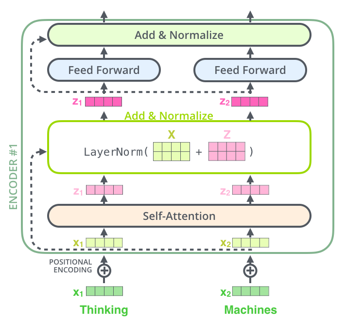
The purpose of the Normalize layer is to normalize the input data, converting it into data with a mean of 0 and a variance of 1. LN calculates the mean and variance on each sample, as shown in the diagram below:
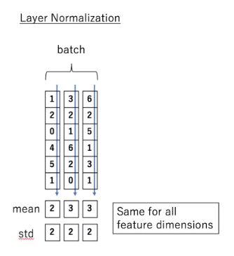
LN’s formula is as follows:
LN(x_i) = α * (x_i – μ_L / √(σ^2_L + ε)) + β
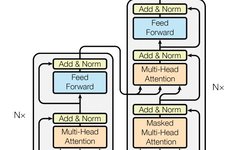
This concludes the content of the encoder layer. Finally, here is an internal diagram showing two stacked encoders:
03
Application Tasks and Results
3.1 NLP Field
In machine translation and NLP, the transformer model based on the attention mechanism has achieved good results, but since the focus is on the CV field, it will not be elaborated here.
3.2 CV Field
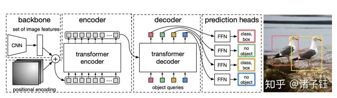
3.2.1 Detection DETR
The first paper to use transformers for end-to-end object detection:
End to End Object Detection With Transformer [3]
First, features are extracted using CNN, and then each point in the final feature map is treated as a word, transforming the feature map into a sequence of words, while the output of the detection is a set of objects, making transformer suitable for this task.
This article builds an end-to-end object detection model using a complete transformer and also discards the manually designed anchor method, proposing a new loss function. However, the focus remains on the model structure. The model structure is illustrated in the diagram below:
This paper has the following highlights:
-
No NMS, directly performing set prediction.
-
Binary graph matching loss.
-
Object queries are interesting, as they are meaningless information by themselves.
Experimental results show that this model can achieve results comparable to those of the rigorously tuned Faster R-CNN baseline. The DETR model is simple and direct, but its drawbacks include long training times and poor detection performance for small targets.
3.2.2 Classification ViT
An Image Is Worth 16X16 Words: Transformers for Image Recognition at Scale[2]
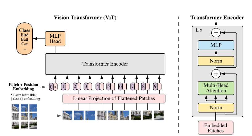
This article differs from previous work by attempting to transfer the NLP transformer to the CV field without modifications. However, the language data processed in NLP is serialized, while the image data processed in CV is three-dimensional (height, width, and channels). Therefore, some method is needed to convert the three-dimensional image data into serialized data. In the article, images are cut into patches, and these patches are arranged in a certain order, forming serialized data.
Based on this, the author proposes the Vision Transformer model.
This paper first attempts to apply the Transformer model to the image classification task with minimal modifications, and the results obtained on ImageNet are inferior to those of ResNet. This is due to the Transformer model’s lack of inductive bias, such as translational invariance and locality like CNNs, which hampers its generalization to the task when data is insufficient.
However, as the training data volume increases, the inductive bias issue can be mitigated, meaning that if trained on a sufficiently large dataset, it can transfer well to smaller datasets.
In experiments, the authors found that on medium-sized datasets (e.g., ImageNet), the transformer model performs worse than ResNets; however, as the dataset size increases, the transformer model’s performance approaches or exceeds some current SOTA results. **The authors believe that large-scale training encourages transformers to learn the translation equivariance and locality that CNN structures possess.
3.2.3 Segmentation SETR
Rethinking Semantic Segmentation from a Sequence-to-Sequence Perspective with Transformers
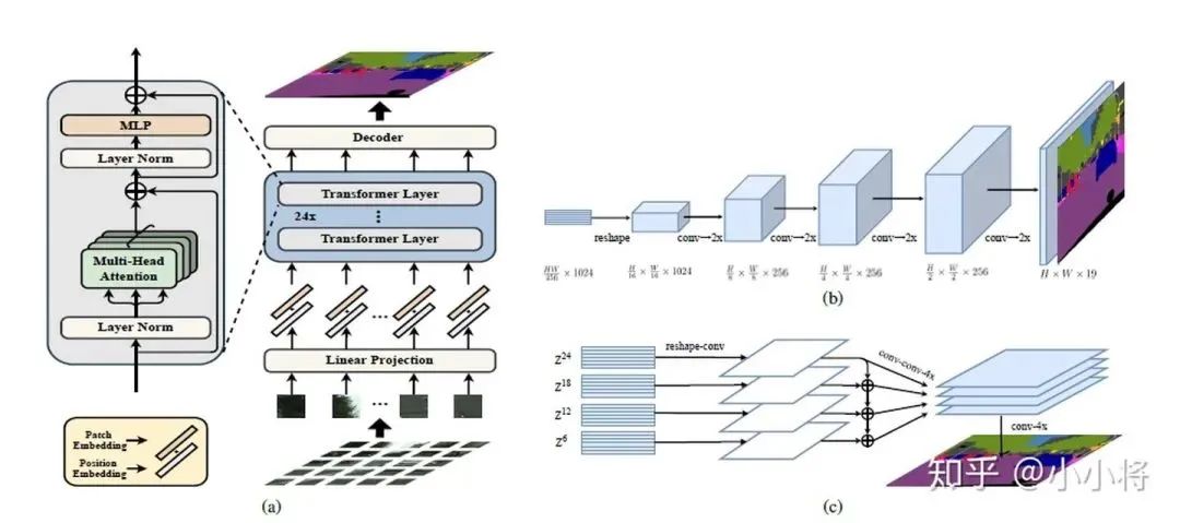
Using ViT as the image encoder, and then adding a CNN decoder to complete the prediction of the semantic map.
A large number of experiments show that SETR achieves new levels on ADE20K (50.28%mIoU), Pascal Context (55.83%mIoU), and Cityscapes. Particularly, it achieved first place (44.42%mIoU) on the highly competitive ADE20K test server leaderboard.
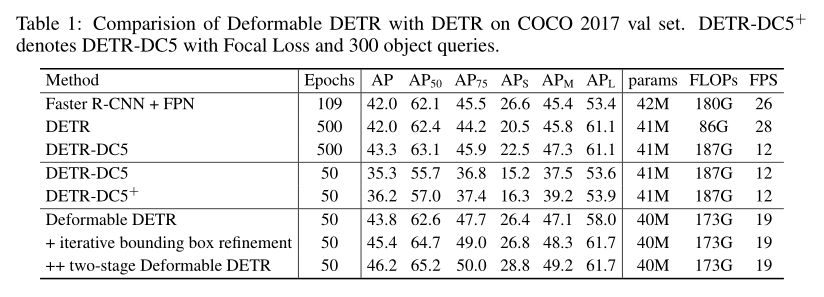
3.2.4 Deformable-DETR
DEFORMABLE DETR: DEFORMABLE TRANSFORMERS FOR END-TO-END OBJECT DETECTION[5]
Improvements over the previous DETR.
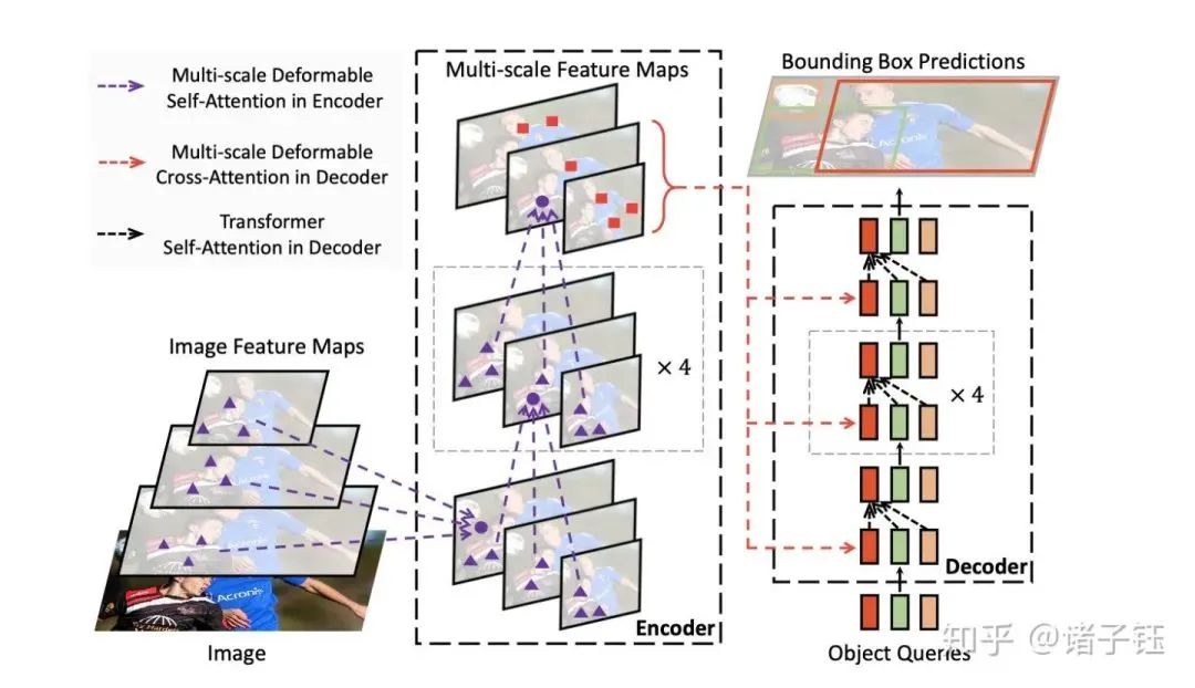
Highlights include:
-
Incorporation of deformable parameters.
-
Multi-scale feature fusion.
Experimental results: reduced training time with improved performance.
04
Advantages and Analysis
1. Compared to RNN, which must compute in chronological order, the significant advantage of Transformer parallel processing mechanism is higher computational efficiency, allowing for significantly faster training speeds, enabling training on larger datasets.
-
For example, GPT-3 (the third generation of Transformer) has a training dataset of approximately 500 billion words, with a model parameter count reaching 175 billion, far exceeding any existing RNN-based models.
-
The algorithm’s parallelism is excellent and aligns well with current hardware (mainly referring to GPUs).
2. The Transformer model also exhibits good scalability and flexibility.
-
In facing specific tasks, a common practice is to first train on large datasets and then fine-tune on specified task datasets. Moreover, as the model size and dataset grow, the model’s performance also improves, and so far, there has been no apparent performance ceiling.
3. The feature extraction capability of the Transformer is superior to that of RNN series models.
4. The design of the Transformer is innovative enough, as it discards the fundamental RNN or CNN in NLP and achieves very good results. The algorithm’s design is truly remarkable, deserving careful study and appreciation by anyone involved in deep learning.
5. The key to the performance improvement brought about by the Transformer design is transforming the distance between any two words into 1, which is highly effective in addressing the long-term dependency issues in NLP.
6. The Transformer can be applied not only in the NLP machine translation field but also has great research potential in other domains.
The characteristics of the Transformer not only led to its success in NLP but also provide the potential for transferring it to other tasks.
05
Disadvantages and Analysis
1. The Transformer model lacks inductive bias, such as not possessing translational invariance and locality like CNNs, which means it cannot generalize well to tasks when data is insufficient.
However, as the training data volume increases, the inductive bias issue can be alleviated, meaning that if trained on a sufficiently large dataset, it can transfer well to smaller datasets.
2. The blunt abandonment of RNN and CNN, while impressive, also causes the model to lose the ability to capture local features. A combination of RNN + CNN + Transformer may yield better results.
3. The loss of positional information in the Transformer is crucial in NLP, and the paper’s addition of Position Embedding in the feature vector is merely a stopgap, failing to rectify the inherent flaws in the Transformer structure.
06
References