Understanding Self-Attention Mechanism: 8 Steps with Code

Originally from New Machine Vision

BERT, RoBERTa, ALBERT, SpanBERT, DistilBERT, SesameBERT, SemBERT, MobileBERT, TinyBERT, CamemBERT… What do they have in common? The answer is not “They are all BERT” 🤭.

The correct answer is: self-attention 🤗.

We are discussing not just the architecture named “BERT”, but more accurately, the Transformer-based architecture. Transformer-based architectures are primarily used for modeling language understanding tasks, avoiding the use of recursion in neural networks, and completely relying on the self-attention mechanism to map the global dependencies between inputs and outputs. But what are the mathematical principles behind this?

This is what this article aims to explain. It will take you through a self-attention module and the mathematical operations involved. By the end of this article, you will be able to write a self-attention module from scratch.

Let’s get started!

What is self-attention?

If you think self-attention is similar to attention, the answer is yes! They essentially share the same concepts and many common mathematical operations.

A self-attention module receives n inputs and returns n outputs. What happens in this module? In layman’s terms, the self-attention mechanism allows inputs to interact with each other (“self”) and find out what they should pay more attention to (“attention”). The output is the sum of these interactions and attention scores.

Writing a self-attention module involves the following steps:

• Prepare Inputs

• Initialize Weights

• Derive Key, Query, and Value

• Compute Attention Scores for Input 1

• Calculate Softmax

• Multiply Scores with Values

• Sum Weighted Values to Get Output 1

• Repeat Steps 4-7 for Inputs 2 and 3

Note: In reality, the mathematical operations are vectorized, meaning all inputs undergo the mathematical operations together. This can be seen in the code section later.

Step 1: Prepare Inputs

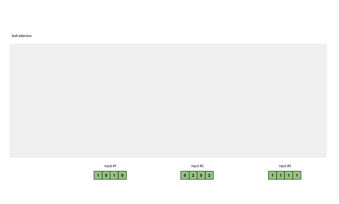
Figure 1.1: Prepare Inputs

In this tutorial, we start with 3 inputs, each with a dimension of 4.

Step 2: Initialize Weights

Each input must have three representations (see below). These representations are called Keys (key, orange), Queries (query, red), and Values (value, purple). In this example, we assume the dimensionality of these representations is 3. Since the dimension of each input is 4, this means each set of weights must be 4×3.

Note: Later we will see that the dimension of the value is also the dimension of the output.

Figure 1.2: Deriving Key, Query, and Value Representations from Each Input

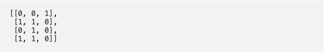
To obtain these representations, each input (green) is multiplied by a set of key weights, a set of query weights, and a set of value weights. In this example, we will initialize the three sets of weights as follows.

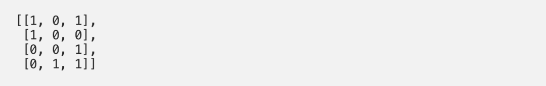
Weights for Key:

Weights for Query:

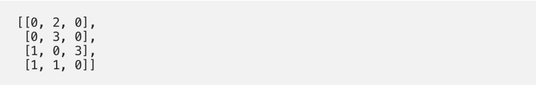
Weights for Value:

Note: In a neural network setting, these weights are usually small numbers, randomly initialized using an appropriate distribution (e.g., Gaussian, Xavier, and Kaiming distributions).

Step 3: Derive Keys, Queries, and Values

Now that we have three sets of weights, let’s actually obtain the key, query, and value representations for each input.

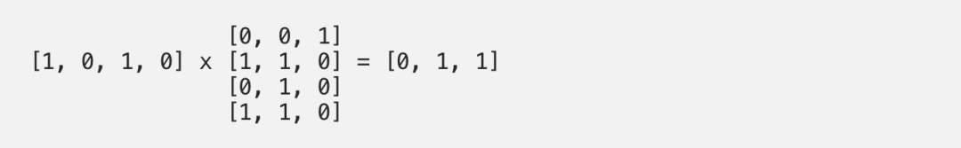
Key representation for Input 1:

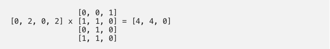
Using the same set of weights to obtain the key representation for Input 2:

Using the same set of weights to obtain the key representation for Input 3:

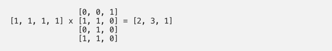
A faster way is to vectorize the above operations:

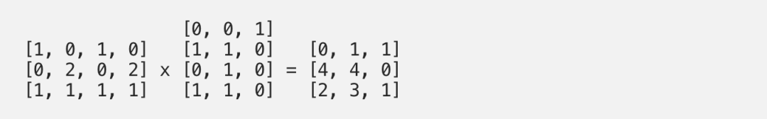
Figure 1.3a: Deriving Key Representations from Each Input

In the same way, we can obtain the value representations for each input:

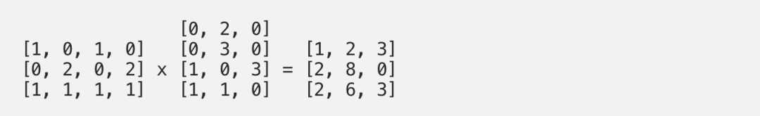
Figure 1.3b: Deriving Value Representations from Each Input

Finally, we obtain the query representation:

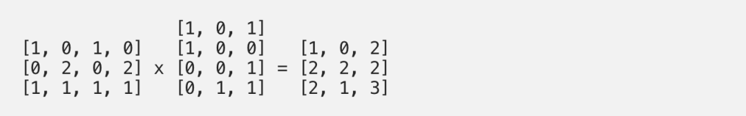
Figure 1.3b: Deriving Query Representations from Each Input

Note: In practice, a bias vector can be added to the product of the matrix multiplication.

Step 4: Compute Attention Scores for Input 1

Figure 1.4: Calculating Attention Scores from Query 1 (blue)

To obtain the attention scores, we first take a dot product between the Query (red) of Input 1 and all Keys (orange). Since there are 3 Key representations (because there are 3 inputs), we obtain 3 Attention Scores (blue).

Note: Now we are only using the query from Input 1. Later, we will repeat the same steps for the other queries.

Step 5: Calculate Softmax

Figure 1.5: Softmax Attention Scores (blue)

Applying softmax to all the attention scores (blue).

Step 6: Multiply Scores with Values

Figure 1.6: Deriving Weighted Value Representations from Values (purple) and Scores (blue)

The softmaxed attention scores (blue) of each input are multiplied by their corresponding values (purple). This results in 3 aligned vectors (yellow). In this tutorial, we will refer to them as Weighted Values.

Step 7: Sum Weighted Values to Get Output 1

Figure 1.7: Summing All Weighted Values (yellow) to Get Output 1 (dark green)

Summing all weighted values (yellow) element-wise:

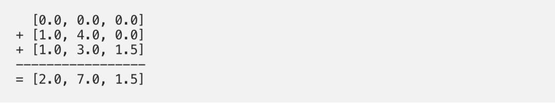
The resulting vector [2.0,7.0,1.5] (dark green) is Output 1, which is based on the query representation of Input 1 interacting with all other keys (including itself).

Step 8: Repeat for Inputs 2 and 3

Now that we have completed Output 1, we repeat Steps 4 to 7 for Outputs 2 and 3. Next, I believe you can handle it on your own 👍🏼.

Figure 1.8: Repeating Steps for Inputs 2 and 3

This is PyTorch code 🤗, a popular deep learning framework for Python.

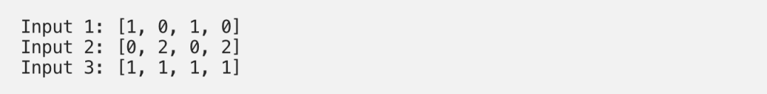
Step 1: Prepare Inputs

import torch
x = [  [1, 0, 1, 0], # Input 1  [0, 2, 0, 2], # Input 2  [1, 1, 1, 1]  # Input 3 ]
x = torch.tensor(x, dtype=torch.float32)

Step 2: Initialize Weights

w_key = [  [0, 0, 1],  [1, 1, 0],  [0, 1, 0],  [1, 1, 0]]
w_query = [  [1, 0, 1],  [1, 0, 0],  [0, 0, 1],  [0, 1, 1]]
w_value = [  [0, 2, 0],  [0, 3, 0],  [1, 0, 3],  [1, 1, 0]]
w_key = torch.tensor(w_key, dtype=torch.float32)
w_query = torch.tensor(w_query, dtype=torch.float32)
w_value = torch.tensor(w_value, dtype=torch.float32)

Step 3: Derive Keys, Queries, and Values

keys = x @ w_key
querys = x @ w_query
values = x @ w_value
print(keys)
# tensor([[0., 1., 1.],
#         [4., 4., 0.],
#         [2., 3., 1.]])
print(querys)
# tensor([[1., 0., 2.],
#         [2., 2., 2.],
#         [2., 1., 3.]])
print(values)
# tensor([[1., 2., 3.],
#         [2., 8., 0.],
#         [2., 6., 3.]])

Step 4: Calculate Attention Scores

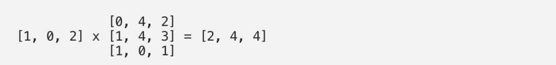
attn_scores = querys @ keys.T
# tensor([[ 2.,  4.,  4.],  # attention scores from Query 1
#         [ 4., 16., 12.],  # attention scores from Query 2
#         [ 4., 12., 10.]]) # attention scores from Query 3

Step 5: Calculate Softmax

from torch.nn.functional import softmax
attn_scores_softmax = softmax(attn_scores, dim=-1)
# tensor([[6.3379e-02, 4.6831e-01, 4.6831e-01],
#         [6.0337e-06, 9.8201e-01, 1.7986e-02],
#         [2.9539e-04, 8.8054e-01, 1.1917e-01]])
# For readability, approximate the above as follows
attn_scores_softmax = [  [0.0, 0.5, 0.5],  [0.0, 1.0, 0.0],  [0.0, 0.9, 0.1]]
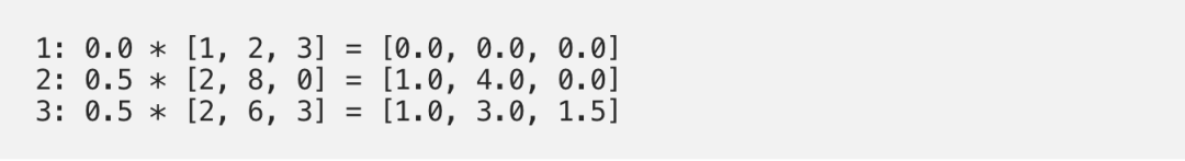
attn_scores_softmax = torch.tensor(attn_scores_softmax)

Step 6: Multiply Scores with Values

weighted_values = values[:,None] * attn_scores_softmax.T[:,:,None]
# tensor([[[0.0000, 0.0000, 0.0000],
#          [0.0000, 0.0000, 0.0000],
#          [0.0000, 0.0000, 0.0000]],
# #         [[1.0000, 4.0000, 0.0000],
#          [2.0000, 8.0000, 0.0000],
#          [1.8000, 7.2000, 0.0000]],
# #         [[1.0000, 3.0000, 1.5000],
#          [0.0000, 0.0000, 0.0000],
#          [0.2000, 0.6000, 0.3000]]])

Step 7: Sum Weighted Values

outputs = weighted_values.sum(dim=0)
# tensor([[2.0000, 7.0000, 1.5000],  # Output 1
#         [2.0000, 8.0000, 0.0000],  # Output 2
#         [2.0000, 7.8000, 0.3000]]) # Output 3

So, what’s next? Transformers!

Indeed, we live in an exciting era of deep learning research and high computational resources. Transformers were proposed in “Attention is All You Need”, originally used for performing neural machine translation. Researchers have reorganized, cut, added, and extended upon it, applying it to more language tasks.

Here, I will briefly introduce how to extend self-attention to the Transformer architecture.

In the self-attention module:

• Dimension

• Bias

Inputs to the self-attention module:

• Embedding module

• Positional encoding

• Truncating

• Masking

Add more self-attention modules:

• Multihead

• Layer stacking

• Modules between self-attention modules:

• Linear transformations

• LayerNorm

That’s all! I hope you find the content simple and easy to understand.

References:

Attention Is All You Need

https://arxiv.org/abs/1706.03762

The Illustrated Transformer

https://jalammar.github.io/illustrated-transformer/

[Disclaimer] The reproduction is for educational and research purposes only, aimed at disseminating academic news information. Copyright belongs to the original author. If there is any infringement, please contact us immediately, and we will delete it promptly.