Normalization Techniques Evolution: In-Depth Analysis of Six Key PyTorch Normalization Layers

This article is about 4200 words long, recommended reading time is over 10 minutes.
This article provides a detailed introduction to several key normalization techniques in deep learning.

Normalization is a key concept in deep learning that ensures faster convergence, more stable training, and better overall performance. PyTorch includes several normalization layers, and we will take a detailed look at the function and usage of each normalization layer.

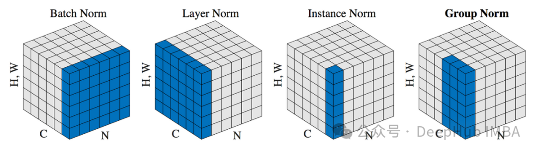
BN

Batch Normalization (BN) is a widely used technique for accelerating the training of deep neural networks and improving their performance. It normalizes the input of each mini-batch of data, keeping the inputs to the intermediate layers of the network relatively stable, which helps to address the issues of vanishing or exploding gradients during training.

import torch.nn as nn
norm = nn.BatchNorm2d(num_features=64)

Key Functions of Batch Normalization:

• Improving Gradient Flow: By normalizing the inputs of the layers, batch normalization helps to pass gradients more smoothly, which is especially important when training deep networks.
• Allowing Higher Learning Rates: Due to the effect of normalization, the parameter space becomes smoother, allowing for higher learning rates without causing instability in the training process.
• Reducing Sensitivity to Initialization: Normalization reduces the impact of initial weight settings, making the training process more stable.

• Having a Slight Regularization Effect: The noise introduced by estimating the mean and variance for each mini-batch can be seen as a slight form of regularization, helping to prevent overfitting.

Workflow of Batch Normalization:

During training, batch normalization achieves normalization through the following steps:

• Calculating Batch Mean and Variance: For the given mini-batch of data, calculate the mean and variance of its features.
• Normalization: Use the calculated mean and variance to normalize each feature in the mini-batch, ensuring that the output has a mean close to 0 and variance close to 1.

• Scaling and Shifting: The normalized data is scaled and shifted using learnable parameters, which are learned during training, allowing the model to recover useful features that may have been removed by the normalization operation.

During model inference or testing, the mean and variance are no longer calculated in real-time for each mini-batch, but instead use the moving averages from the entire training set.

Batch normalization has become a fundamental component in building modern deep learning models, especially when dealing with convolutional networks and deep fully connected networks.

LN

Layer Normalization (LN) is a technique that standardizes the inputs of each layer in a neural network. It shares a similar purpose with batch normalization, aiming to help neural networks learn faster and more stably. Unlike batch normalization, which normalizes the same features across multiple data samples in a mini-batch, layer normalization normalizes all or part of the features within a single sample.

import torch.nn as nn
norm = nn.LayerNorm(256)

Main Characteristics of Layer Normalization:

• Independent of Batch Size: The operation of layer normalization is independent of the batch size, making it particularly useful in situations where the batch size varies significantly or is 1 (common in online learning and reinforcement learning).
• Applicable to Recurrent Structures: In Recurrent Neural Networks (RNNs), batch normalization is difficult to apply effectively due to dependencies between time steps. Layer normalization, being independent of the batch dimension, can be better applied in RNNs and their variants.

• Simplifying Model Training: Since layer normalization does not depend on batch statistics, its behavior during training and inference is more consistent, simplifying model deployment and maintenance.

Working Principle of Layer Normalization:

Layer normalization is typically implemented in the hidden layers of neural networks, with the following steps:

• Calculating Feature Statistics: For each training sample, calculate the mean and variance of all or part of the neurons in a single layer.
• Normalization: Use the calculated mean and variance to normalize each feature in each sample, ensuring that the mean is 0 and the variance is 1.

• Reparameterization: By introducing learnable scaling and shifting parameters, the normalized output is adjusted, allowing the network to utilize these parameters to recover information that may be useful for the learning task.

Layer normalization is particularly effective in Transformer models used in natural language processing (e.g., BERT, GPT, etc.). By applying layer normalization in each hidden layer, these models can train deep network structures more effectively.

IN

Instance Normalization (IN) is a normalization technique specific to the field of image processing, especially widely used in style transfer and Generative Adversarial Networks (GANs). Instance normalization shares similar goals with batch normalization and layer normalization, which is to speed up neural network training and improve performance, but it differs in its approach.

import torch.nn as nn
norm = nn.InstanceNorm2d(num_features=64)

Characteristics of Instance Normalization:

• Targeting Individual Data Instances: Instance normalization operates independently of other samples, normalizing each sample’s channels separately, making it suitable for situations where the batch size is 1.

• Widely Used in Visual Tasks: Instance normalization is particularly effective in visual tasks, especially in style transfer, helping the network learn and transfer style features better without being affected by image content.

Workflow of Instance Normalization:

Instance normalization is primarily applied in convolutional neural networks, with the following steps:

• Calculating Channel Statistics: For each channel in each data instance, calculate the mean and variance of all elements in that channel.
• Normalization: Use the calculated statistics to normalize all pixels in each channel, ensuring the output has a mean of 0 and variance of 1.

• Reparameterization: Similar to other normalization techniques, instance normalization also uses learnable scaling and shifting parameters to adjust the normalized output, allowing the model to recover potentially helpful information for the task.

In the application of image style transfer, instance normalization helps the network focus on learning style features of images rather than content features. This characteristic makes instance normalization perform better than batch normalization in artistic style transfer tasks, as it allows the network to adjust its style representation independently for each image, thus more effectively simulating different artistic styles.

GN

Group Normalization (GN) lies between instance normalization and layer normalization. Group normalization was proposed by He Kaiming et al. in 2018, primarily targeting situations with small batch training data to address the instability issues that batch normalization may bring on small batch data.

import torch.nn as nn
norm = nn.GroupNorm(num_groups=4, num_channels=64)

Characteristics of Group Normalization:

• Independent of Batch Size: Unlike batch normalization, the effectiveness of group normalization does not depend on batch size, making it effective even when the batch is small or consists of a single sample.

• Applicable to Various Network Structures: Group normalization can be applied to various structures, including convolutional neural networks (CNNs) and recurrent neural networks (RNNs), improving the model’s generalization ability and stability.

Working Principle of Group Normalization:

Group normalization divides the features of each sample into several groups, normalizing within each group. Here, a “group” refers to dividing the channels of a sample into several subsets, with mean and variance calculated independently within each subset for normalization.

Specific steps include:

• Grouping: Choose an appropriate number of groups G (usually treated as a hyperparameter). The channels of each sample are evenly distributed among these groups.
• Calculating Mean and Variance: For the channels within each group, calculate the mean and variance of all activation values.
• Normalization: Use the calculated mean and variance to normalize the activation values of each channel within each group.

• Reparameterization: The normalized output is adjusted using learnable scaling and shifting parameters to allow the model to recover potentially useful information for the task.

Group normalization exhibits excellent performance in many deep learning tasks, especially in applications where batch normalization is not suitable (e.g., very small batch sizes). It provides model stability while maintaining high training and inference efficiency. Additionally, due to its independence from batch size, group normalization is particularly suited for applications requiring high real-time performance, such as video processing and real-time applications on mobile devices.

SyncBN

Synchronized Batch Normalization (SyncBN) is a variant of batch normalization primarily applied in multi-GPU training environments. In standard batch normalization, each GPU independently computes the mean and variance for its received data batches, which can affect the normalization effect when the number of GPUs is high, as each GPU may have a small batch size. Synchronized batch normalization addresses this issue by synchronizing the computation of mean and variance across multiple GPUs or devices, effectively increasing the overall batch size and thereby improving the stability and effectiveness of normalization.

import torch.nn as nn
norm = nn.SyncBatchNorm(num_features=64)

Working Principle of Synchronized Batch Normalization:

• Cross-Device Synchronization: During forward and backward propagation, each GPU computes its batch mean and variance, then these statistics are aggregated across all GPUs to compute global mean and variance.
• Global Normalization: Use the aggregated global mean and variance to normalize the data across the GPUs.

• Learning Parameters: The normalized data is adjusted using learnable scaling and shifting parameters, which are optimized during the network training process.

Advantages of Synchronized Batch Normalization:

• Enhancing Model Stability: By using larger global batch statistics, it reduces the inaccuracies in estimates caused by insufficient batch sizes in batch normalization.
• Improving Training Efficiency: In multi-GPU training, SyncBN helps to accelerate the convergence speed and final performance of the network, as the normalization process on each device utilizes information from all devices.

• Suitable for Distributed Training: Particularly suitable for large-scale distributed training, as it balances and unifies training dynamics across different devices.

Synchronized batch normalization is especially suitable for resource-rich training environments, such as those using multiple GPUs or multiple machines for training. This is particularly important when dealing with large networks and complex models (such as large image recognition, video processing, or large-scale language models) that typically require substantial computational resources and data batches to achieve optimal performance.

Synchronized batch normalization effectively overcomes the challenges faced by traditional batch normalization in distributed training by synchronizing the computation of mean and variance in multi-GPU environments, enhancing the effectiveness and efficiency of model training.

LRN

Local Response Normalization (LRN) is a normalization technique applied in convolutional neural networks (CNNs), particularly in earlier deep learning models like AlexNet, used for image recognition tasks. LRN is inspired by the biological phenomenon of lateral inhibition, which enhances the local contrast of patterns by suppressing the neurons around active neurons, improving the neural network’s responsiveness to information in images.

import torch.nn as nn
norm = LocalResponseNorm(size=2)

Local response normalization works by normalizing a given activation within a local neighborhood, which typically consists of different channels at the same spatial location. The specific steps are as follows:

• Calculating Activations: First, calculate the square of the activation values for each channel at a specific location.
• Neighborhood Summation: Sum the square of each activation value within a specified neighborhood, typically including several channels before and after the current channel.
• Normalization: Each activation value is adjusted according to a normalization formula involving the sum of its neighborhood, which includes adjustable parameters to control the extent of normalization.

• Maintaining Proportions: In this way, the output of one neuron is adjusted based on its activity relative to other neurons in the neighborhood, achieving a local suppression effect.

The mathematical formula for LRN is typically represented as:

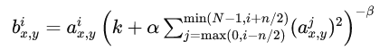
Where:

ax,yi is the original activation value of the i-th channel at position (x, y).

bx,yi is the normalized activation value.

n is the size of the neighborhood.

α, β, k are hyperparameters used to adjust the normalization effect.

N is the total number of channels.

LRN was widely used in some early CNN models, such as AlexNet, to improve classification accuracy. However, with the development of deep learning technology, especially with the emergence of more advanced normalization techniques like batch normalization, the use of LRN has decreased. This is because batch normalization not only provides a more stable and faster training process but also significantly improves the final performance of the model. Therefore, the use of LRN has gradually been replaced by other normalization methods in modern deep learning architectures.

Conclusion

This article provides a detailed introduction to several key normalization techniques in deep learning: Batch Normalization (BN), Layer Normalization (LN), Instance Normalization (IN), Group Normalization (GN), Synchronized Batch Normalization (SyncBN), and Local Response Normalization (LRN). These techniques help improve the learning speed and performance of the network by normalizing the data within neural networks. Each technique is optimized for different application scenarios and needs, such as batch normalization being suitable for large batch data processing, instance normalization primarily used for image style transfer, while group normalization is suitable for small batch data. Synchronized batch normalization optimizes the normalization process for multi-GPU training, while local response normalization, although used more in earlier models, has been less utilized in modern architectures.

Editor: Huang Jiyan

About Us

Data Pie THU, as a public account focused on data science, backed by the Tsinghua University Big Data Research Center, shares cutting-edge data science and big data technology innovation research dynamics, continuously disseminating data science knowledge, striving to build a data talent gathering platform, and creating the strongest group of big data in China.

Sina Weibo: @Data Pie THU

WeChat Video Account: Data Pie THU

Today’s Headlines: Data Pie THU