Implementing Denoising Diffusion Probabilistic Model (DDPM) from Scratch in PyTorch

Source: DeepHub IMBA


This article is approximately 6500 words long and is recommended to be read in 13 minutes.
This article will build a basic unconditional diffusion model, namely the Denoising Diffusion Probabilistic Model (DDPM).

Diffusion models are typically a type of generative deep learning model that creates data by learning the denoising process. There are many variants of diffusion models, the most popular of which are conditional text models that can generate specific images based on prompts. Some diffusion models (like Control-Net) can even blend images with certain artistic styles.

In this article, we will construct a basic unconditional diffusion model, namely the Denoising Diffusion Probabilistic Model (DDPM). We will start by exploring the intuitive workings of the algorithm, and then build it from scratch in PyTorch. This article mainly focuses on the ideas behind the algorithm and the specific implementation details.

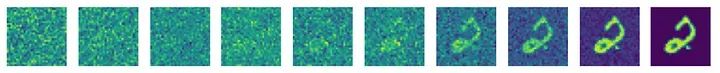
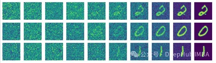
We first show the results of this article, using the diffusion model to generate digits for MNIST.

Principle of Diffusion Models

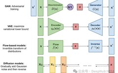
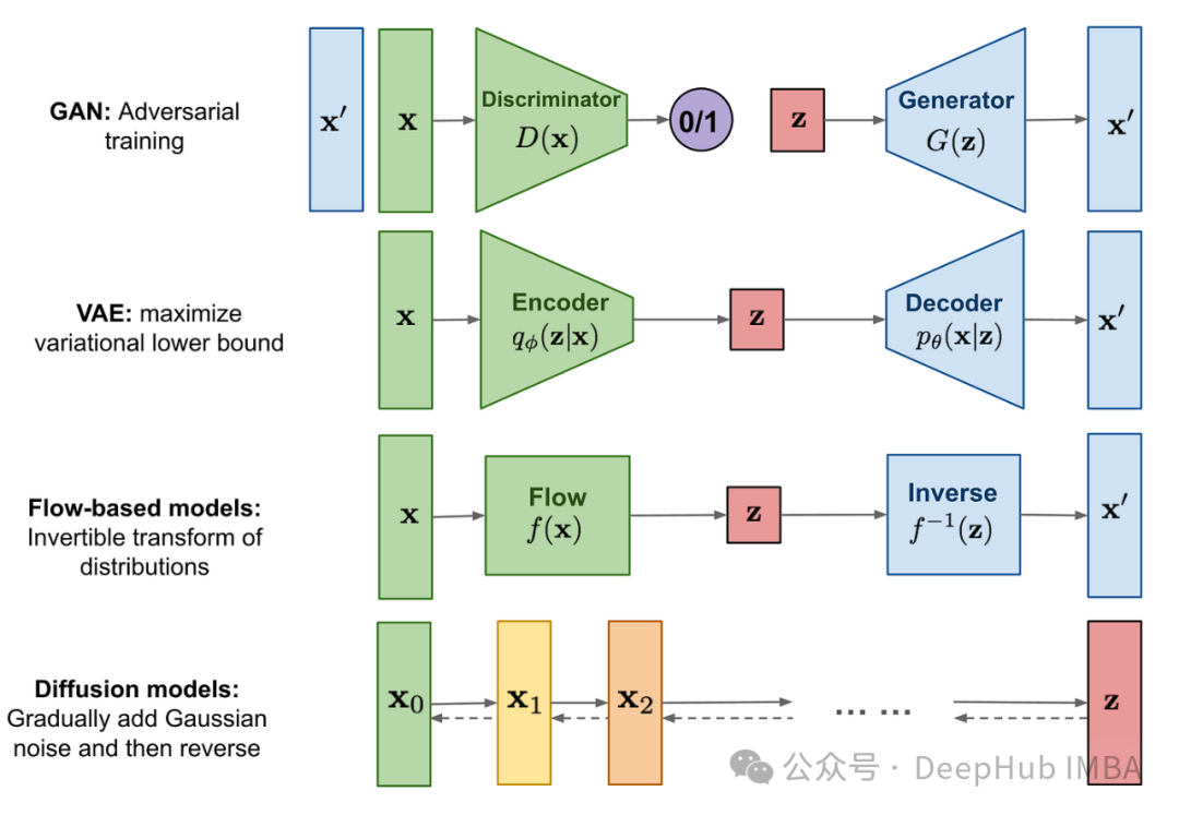
The diffusion process consists of a forward process and a reverse process. The forward process is a predetermined Markov chain based on a noise schedule. The noise schedule is a set of variances B1, B2, … BT that control the conditional normal distributions that make up the Markov chain.

The mathematical expression of the forward process represents the forward process, but intuitively we can understand it as a sequence that gradually maps the data example X to pure noise. At the intermediate time step t, we obtain a noisy version of X, and at the final time step T, we reach pure noise that is approximately controlled by the standard normal distribution. When constructing the diffusion model, we need to choose our noise schedule. For example, in DDPM, the noise schedule features 1000 time steps of linearly increasing variance from 1e-4 to 0.02. It is also important to note that the forward process is static, which means we choose the noise schedule as a hyperparameter of the diffusion model, and this forward process does not require training since it is already clearly defined.

The last key detail about the forward process is that because these distributions are normal, a distribution known as the “diffusion kernel” can be mathematically derived, which is the distribution of any intermediate value in the forward process given the initial data point. This allows us to bypass all intermediate steps of progressively adding t-1 levels of noise in the forward process and directly obtain images with t noise, which will be very convenient during later training of the model. This is mathematically represented as:

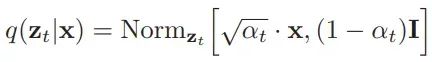
Here, the alpha of time t is defined as the cumulative (1-B) from the initial time step to the current time step.

The reverse process is the key to the diffusion model. Essentially, it is the process of generating a new image from a pure noise image by gradually removing noise. Starting from pure noise data, for each time step t, we subtract the amount of noise theoretically added by the forward process at that time step. By continuing to remove noise, we eventually obtain something similar to the original data distribution. Therefore, our main task is to train a model to approximate the forward process and estimate a reverse process that can generate new samples.

To train such a model to estimate the reverse diffusion process, we can follow the algorithm defined below:

1. Randomly sample a data point from the training dataset.

2. Select a random time step in the noise (variance) schedule.

3. Add the noise of that time step to the data, simulating the forward diffusion process through the “diffusion kernel”.

4. Pass the diffusion image to the model and predict the added noise.

5. Calculate the mean squared error between the predicted noise and the actual noise, and optimize the model’s parameters through this objective function.

6. Repeat the above steps!

Through this method, the model gradually learns how to effectively remove noise, ultimately being able to recover images similar to the original data from almost complete noise. This training objective not only helps the model learn to accurately predict noise but also optimizes its ability to denoise at each time step, making the reverse process more accurate and efficient.

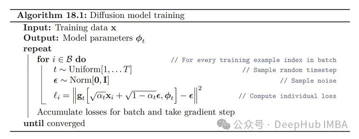
In the algorithm, if we do not look at the complete derivation process, the mathematical formulas may initially seem a bit strange, but intuitively, it is a reparameterization of the diffusion kernel based on the alpha value of the noise schedule, simply put, it is the square difference between the predicted noise and the actual noise added to the image.

If our model can successfully predict the amount of noise based on a specific time step of the forward process, then we can start from the noise at time step T and gradually remove the noise at each time step until we recover a generated sample similar to the original data distribution.

The sampling algorithm can be summarized as follows:

1. Generate random noise from the standard normal distribution.

For each time step moving backwards from the last time step:

2. Update Z by estimating the reverse process distribution, where the mean of this distribution is parameterized by the previous Z and the variance is parameterized by the noise estimated by the model at that time step.

3. For stability, add a small amount of noise back to the image (the reason will be explained below).

4. Repeat the above steps until reaching time step 0, thus obtaining the recovered image!

The key to this process is to precisely adjust the removal of noise at each step, simulating the reverse diffusion, thereby gradually approaching the distribution of the original data. The purpose of adding a small amount of noise is to prevent potential numerical instability that may occur during the denoising process, helping the model to more smoothly reverse map to the original data.

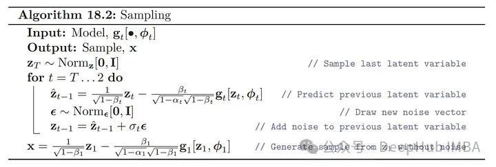
Although the algorithm for generating images appears mathematically complex, intuitively, it boils down to an iterative process where we start from pure noise, estimate the noise theoretically added at time step t, and subtract it. We continue doing this until we obtain our generated sample. One small detail to note is that after we subtract the estimated noise, we add back a small amount of noise to maintain the stability of the process. For example, estimating and subtracting all the noise at once at the beginning would lead to very incoherent samples, so in practice, adding back a bit of noise and iterating through each time step has been empirically shown to generate better samples.

In this process, the core idea is to gradually remove the estimated noise at each time step and then appropriately reintroduce a portion of noise to avoid potential instability in the process. The iteration not only helps to recover more accurate images but also ensures the coherence and usability of the image quality during the generation process. Although the reintroduction of noise at each step may seem counterintuitive, in practice, this strategy is crucial for maintaining the stability of the entire process and is a key step in achieving high-quality image generation.

Unet

In the study of DDPM (Denoising Diffusion Probabilistic Model), the authors used the UNET architecture originally designed for medical image segmentation to construct the model and predict the noise during the reverse diffusion process. In this article, we will use images of 32×32 pixels, and MNIST is such a dataset, but this model can also be extended to handle higher resolution data. UNET has many variants, but the overview of the model architecture we will build is shown in the following figure.

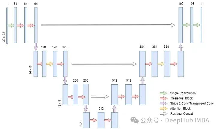
UNET is a deep learning network with a symmetric encoder-decoder structure. The encoder progressively reduces the spatial dimensions of the image while increasing the number of channels, capturing deep features in the image. The decoder does the opposite, progressively restoring the spatial dimensions of the image and reducing the number of channels, ultimately outputting a result of the same size as the input image. In this process, there are skip connections between the encoder and decoder, which help the decoder better restore image details.

This architecture is very suitable for image generation tasks because it can effectively handle and reconstruct details in images. In the diffusion model, the task of UNET is to predict the noise added to the image at each step, which is crucial for the success of the model’s reverse denoising process. In this way, UNET can gradually reduce noise and ultimately restore a clear image.

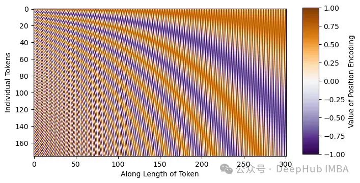
The main difference between DDPM UNET and the classic UNET is that the DDPM UNET incorporates attention mechanisms in the 16×16 dimension layers and adds sinusoidal transformer embeddings in each residual block. The significance of the sinusoidal embedding is to inform the model which time step’s noise we are trying to predict. By injecting positional information into the noise schedule, it helps the model predict the noise at each time step. For example, if our noise schedule has a lot of noise at certain time steps, the model’s understanding of the time step it must predict can help it predict the noise at the corresponding time step.

Sinusoidal embeddings are different sine and cosine frequencies that can be directly added to the input, giving the model extra positional/sequence understanding. As can be seen from the image below, each sine wave is unique, which will make the model aware of its position in our noise schedule.

Model Code Implementation

In our model implementation, we will start by defining our imports and coding the sinusoidal time step embeddings.

 # Imports import torch import torch.nn as nn import torch.nn.functional as F from einops import rearrange #pip install einops from typing import List import random import math from torchvision import datasets, transforms from torch.utils.data import DataLoader from timm.utils import ModelEmaV3 #pip install timm from tqdm import tqdm #pip install tqdm import matplotlib.pyplot as plt #pip install matplotlib import torch.optim as optim import numpy as np
 class SinusoidalEmbeddings(nn.Module):     def __init__(self, time_steps:int, embed_dim: int):         super().__init__()         position = torch.arange(time_steps).unsqueeze(1).float()         div = torch.exp(torch.arange(0, embed_dim, 2).float() * -(math.log(10000.0) / embed_dim))         embeddings = torch.zeros(time_steps, embed_dim, requires_grad=False)         embeddings[:, 0::2] = torch.sin(position * div)         embeddings[:, 1::2] = torch.cos(position * div)         self.embeddings = embeddings
     def forward(self, x, t):         embeds = self.embeddings[t].to(x.device)         return embeds[:, :, None, None]

Each residual block in UNET will use the same parameters as those used in the original DDPM paper. Each residual block will consist of the following series of components:

1. Group Normalization:This normalization technique is a variant of batch normalization used to control internal covariate shift, especially suitable for small batch sizes.

2. ReLU Activation Function:This is a nonlinear activation function that allows the model to capture complex patterns and nonlinear relationships in the input data.

3. 3×3 ‘Same’ Convolution:This convolution operation maintains the spatial dimensions of the output feature map the same as the input, achieved through appropriate padding.

4. Dropout:This is a regularization technique that prevents the model from overfitting by randomly dropping (i.e., setting to zero) some activation units in the network during training.

5. Skip Connection:This connection directly passes the output of a previous layer to a later layer, helping to address the vanishing gradient problem in deep networks and allowing the model to retain information about primary features in deep layers.

 # Residual Blocks class ResBlock(nn.Module):     def __init__(self, C: int, num_groups: int, dropout_prob: float):         super().__init__()         self.relu = nn.ReLU(inplace=True)         self.gnorm1 = nn.GroupNorm(num_groups=num_groups, num_channels=C)         self.gnorm2 = nn.GroupNorm(num_groups=num_groups, num_channels=C)         self.conv1 = nn.Conv2d(C, C, kernel_size=3, padding=1)         self.conv2 = nn.Conv2d(C, C, kernel_size=3, padding=1)         self.dropout = nn.Dropout(p=dropout_prob, inplace=True)
     def forward(self, x, embeddings):         x = x + embeddings[:, :x.shape[1], :, :]         r = self.conv1(self.relu(self.gnorm1(x)))         r = self.dropout(r)         r = self.conv2(self.relu(self.gnorm2(r)))         return r + x

In DDPM, the authors used two residual blocks at each layer (resolution scale) of UNET, and incorporated the classic attention mechanism between the two residual blocks in the 16×16 dimension layers. Below we will implement this attention mechanism for UNET:

 class Attention(nn.Module):     def __init__(self, C: int, num_heads:int , dropout_prob: float):         super().__init__()         self.proj1 = nn.Linear(C, C*3)         self.proj2 = nn.Linear(C, C)         self.num_heads = num_heads         self.dropout_prob = dropout_prob
     def forward(self, x):         h, w = x.shape[2:]         x = rearrange(x, 'b c h w -> b (h w) c')         x = self.proj1(x)         x = rearrange(x, 'b L (C H K) -> K b H L C', K=3, H=self.num_heads)         q,k,v = x[0], x[1], x[2]         x = F.scaled_dot_product_attention(q,k,v, is_causal=False, dropout_p=self.dropout_prob)         x = rearrange(x, 'b H (h w) C -> b h w (C H)', h=h, w=w)         x = self.proj2(x)         return rearrange(x, 'b h w C -> b C h w')

When implementing the attention mechanism, the processing of data is relatively straightforward. We reshape the data so that the height (h) and width (w) dimensions merge into a “sequence” dimension, similar to the input of traditional Transformer models, while the channel dimension becomes the embedding feature dimension. Using torch.nn.functional.scaled_dot_product_attention, because this implementation includes flash attention, which is an optimized version of attention mathematically equivalent to classic attention. Define a complete layer of UNET:

 class UnetLayer(nn.Module):     def __init__(self,             upscale: bool,             attention: bool,             num_groups: int,             dropout_prob: float,             num_heads: int,             C: int):         super().__init__()         self.ResBlock1 = ResBlock(C=C, num_groups=num_groups, dropout_prob=dropout_prob)         self.ResBlock2 = ResBlock(C=C, num_groups=num_groups, dropout_prob=dropout_prob)         if upscale:             self.conv = nn.ConvTranspose2d(C, C//2, kernel_size=4, stride=2, padding=1)         else:             self.conv = nn.Conv2d(C, C*2, kernel_size=3, stride=2, padding=1)         if attention:             self.attention_layer = Attention(C, num_heads=num_heads, dropout_prob=dropout_prob)
     def forward(self, x, embeddings):         x = self.ResBlock1(x, embeddings)         if hasattr(self, 'attention_layer'):             x = self.attention_layer(x)         x = self.ResBlock2(x, embeddings)         return self.conv(x), x

In DDPM, each layer contains two residual blocks and may include an attention mechanism, in addition to passing embeddings to each residual block. The returned downsampled or upsampled values, along with the previous values, will be stored and used for residual concatenation in skip connections.

Complete the UNET class as follows:

 class UNET(nn.Module):     def __init__(self,             Channels: List = [64, 128, 256, 512, 512, 384],             Attentions: List = [False, True, False, False, False, True],             Upscales: List = [False, False, False, True, True, True],             num_groups: int = 32,             dropout_prob: float = 0.1,             num_heads: int = 8,             input_channels: int = 1,             output_channels: int = 1,             time_steps: int = 1000):         super().__init__()         self.num_layers = len(Channels)         self.shallow_conv = nn.Conv2d(input_channels, Channels[0], kernel_size=3, padding=1)         out_channels = (Channels[-1]//2)+Channels[0]         self.late_conv = nn.Conv2d(out_channels, out_channels//2, kernel_size=3, padding=1)         self.output_conv = nn.Conv2d(out_channels//2, output_channels, kernel_size=1)         self.relu = nn.ReLU(inplace=True)         self.embeddings = SinusoidalEmbeddings(time_steps=time_steps, embed_dim=max(Channels))         for i in range(self.num_layers):             layer = UnetLayer(                 upscale=Upscales[i],                 attention=Attentions[i],                 num_groups=num_groups,                 dropout_prob=dropout_prob,                 C=Channels[i],                 num_heads=num_heads            )             setattr(self, f'Layer{i+1}', layer)
     def forward(self, x, t):         x = self.shallow_conv(x)         residuals = []         for i in range(self.num_layers//2):             layer = getattr(self, f'Layer{i+1}')             embeddings = self.embeddings(x, t)             x, r = layer(x, embeddings)             residuals.append(r)         for i in range(self.num_layers//2, self.num_layers):             layer = getattr(self, f'Layer{i+1}')             x = torch.concat((layer(x, embeddings)[0], residuals[self.num_layers-i-1]), dim=1)         return self.output_conv(self.relu(self.late_conv(x)))

The only difference in this implementation compared to the original text is that the upstream channels are slightly larger than the typical channels of UNET. This architecture trains more efficiently on a single GPU with 16GB VRAM.

Scheduler

Writing a noise/variance scheduler for DDPM is also very simple. In DDPM, our scheduler will start at 1e-4, end at 0.02, and increase linearly.

 class DDPM_Scheduler(nn.Module):     def __init__(self, num_time_steps: int=1000):         super().__init__()         self.beta = torch.linspace(1e-4, 0.02, num_time_steps, requires_grad=False)         alpha = 1 - self.beta         self.alpha = torch.cumprod(alpha, dim=0).requires_grad_(False)
     def forward(self, t):         return self.beta[t], self.alpha[t]

It returns both the beta (variance) value and the alpha value, as both the training and sampling formulas are based on their mathematical derivations.

This function finally defines a random seed. If you want to reproduce a specific training instance, using the same seed each time ensures that the random weights and optimizer initialization are the same.

 def set_seed(seed: int = 42):     torch.manual_seed(seed)     torch.cuda.manual_seed_all(seed)     torch.backends.cudnn.deterministic = True     torch.backends.cudnn.benchmark = False     np.random.seed(seed)     random.seed(seed)

Training Code

For our implementation, we will create a model to generate MNIST data (handwritten digits). Since these images are by default 28×28 in PyTorch, we will pad the images to 32×32 to conform to the standard of the original paper that trained on 32×32 images.

Using the Adam optimizer, the initial learning rate is set to 2e-5. We also use EMA (Exponential Moving Average) to help improve generation quality. EMA is a weighted average of the model parameters that can create smoother, less noisy samples during inference. In this implementation, we use the EMA V3 implementation from the timm library, with the weight set to 0.9999, the same as used in the DDPM paper.

 def train(batch_size: int=64,           num_time_steps: int=1000,           num_epochs: int=15,           seed: int=-1,           ema_decay: float=0.9999,             lr=2e-5,           checkpoint_path: str=None):     set_seed(random.randint(0, 2**32-1)) if seed == -1 else set_seed(seed)
     train_dataset = datasets.MNIST(root='./data', train=True, download=False,transform=transforms.ToTensor())     train_loader = DataLoader(train_dataset, batch_size=batch_size, shuffle=True, drop_last=True, num_workers=4)
     scheduler = DDPM_Scheduler(num_time_steps=num_time_steps)     model = UNET().cuda()     optimizer = optim.Adam(model.parameters(), lr=lr)     ema = ModelEmaV3(model, decay=ema_decay)     if checkpoint_path is not None:         checkpoint = torch.load(checkpoint_path)         model.load_state_dict(checkpoint['weights'])         ema.load_state_dict(checkpoint['ema'])         optimizer.load_state_dict(checkpoint['optimizer'])     criterion = nn.MSELoss(reduction='mean')
     for i in range(num_epochs):         total_loss = 0         for bidx, (x,_) in enumerate(tqdm(train_loader, desc=f"Epoch {i+1}/{num_epochs}")):             x = x.cuda()             x = F.pad(x, (2,2,2,2))             t = torch.randint(0,num_time_steps,(batch_size,))             e = torch.randn_like(x, requires_grad=False)             a = scheduler.alpha[t].view(batch_size,1,1,1).cuda()             x = (torch.sqrt(a)*x) + (torch.sqrt(1-a)*e)             output = model(x, t)             optimizer.zero_grad()             loss = criterion(output, e)             total_loss += loss.item()             loss.backward()             optimizer.step()             ema.update(model)         print(f'Epoch {i+1} | Loss {total_loss / (60000/batch_size):.5f}')
     checkpoint = {         'weights': model.state_dict(),         'optimizer': optimizer.state_dict(),         'ema': ema.state_dict()    }     torch.save(checkpoint, 'checkpoints/ddpm_checkpoint')

Inference

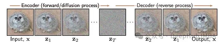
During the inference phase, we simply reverse the forward process. Starting from pure noise, the now-trained model can predict the estimated noise at each time step, and can iteratively generate entirely new samples. From each different noise starting point, a sample similar to the original data distribution but unique can be generated.

 def display_reverse(images: List):     fig, axes = plt.subplots(1, 10, figsize=(10,1))     for i, ax in enumerate(axes.flat):         x = images[i].squeeze(0)         x = rearrange(x, 'c h w -> h w c')         x = x.numpy()         ax.imshow(x)         ax.axis('off')     plt.show()
 def inference(checkpoint_path: str=None,               num_time_steps: int=1000,               ema_decay: float=0.9999, ):     checkpoint = torch.load(checkpoint_path)     model = UNET().cuda()     model.load_state_dict(checkpoint['weights'])     ema = ModelEmaV3(model, decay=ema_decay)     ema.load_state_dict(checkpoint['ema'])     scheduler = DDPM_Scheduler(num_time_steps=num_time_steps)     times = [0,15,50,100,200,300,400,550,700,999]     images = []
     with torch.no_grad():         model = ema.module.eval()         for i in range(10):             z = torch.randn(1, 1, 32, 32)             for t in reversed(range(1, num_time_steps)):                 t = [t]                 temp = (scheduler.beta[t]/( (torch.sqrt(1-scheduler.alpha[t]))*(torch.sqrt(1-scheduler.beta[t])) ))                 z = (1/(torch.sqrt(1-scheduler.beta[t])))*z - (temp*model(z.cuda(),t).cpu())                 if t[0] in times:                     images.append(z)                 e = torch.randn(1, 1, 32, 32)                 z = z + (e*torch.sqrt(scheduler.beta[t]))             temp = scheduler.beta[0]/( (torch.sqrt(1-scheduler.alpha[0]))*(torch.sqrt(1-scheduler.beta[0])) )             x = (1/(torch.sqrt(1-scheduler.beta[0])))*z - (temp*model(z.cuda(),[0]).cpu())
             images.append(x)             x = rearrange(x.squeeze(0), 'c h w -> h w c').detach()             x = x.numpy()             plt.imshow(x)             plt.show()             display_reverse(images)             images = []

Finally, if you need a main function to tie together training and inference, use the following:

 def main():    train(checkpoint_path='checkpoints/ddpm_checkpoint', lr=2e-5, num_epochs=75)    inference('checkpoints/ddpm_checkpoint')
 if __name__ == '__main__':    main()

After training for 75 epochs according to the above code, the following results were obtained:

Conclusion

This concludes our introduction to the implementation process of the Denoising Diffusion Probabilistic Model (DDPM). We first discussed how to create a model for generating MNIST data, including padding images from the default size of 28×28 to 32×32 to conform to the standards of the original paper. In terms of optimization, we chose the Adam optimizer and combined it with Exponential Moving Average (EMA) to improve generation quality.

In the model training section, we followed a series of clear steps, including adding noise to the data, predicting using UNET, and optimizing the error. We also introduced a basic checkpoint mechanism to pause and resume training at different epochs. The inference phase is the reverse forward process, starting from pure noise, where the model gradually predicts and eliminates noise to ultimately generate images that are similar yet unique to the original data distribution.

Additionally, we included an auxiliary function to visualize the diffusion images, helping users intuitively understand the model’s learning of the reverse process. Through this series of implementations and optimizations, DDPM demonstrates its powerful capabilities in image generation and denoising.

Finally, the original DDPM paper: