MLNLP community is a well-known machine learning and natural language processing community in China and abroad, covering NLP master’s and doctoral students, university teachers, and corporate researchers.

The Vision of the Community is to promote communication and progress between the academic and industrial circles of natural language processing and machine learning in China and abroad, especially for beginners.

Reprinted from | Machine Learning Algorithms

In the previous article, we introduced how OpenAI Sora text-to-video model shocked the AI community again, and mentioned that the Sora model is actually a diffusion model + Transformer. This article continues to discuss the development, principles, and code practice of diffusion models.

Principles and Implementation of Diffusion Models in PyTorch

The trigger for diffusion models began with the introduction of DDPM (Denoising Diffusion Probabilistic Model) in 2020. Before delving into the details of how the Denoising Diffusion Probabilistic Model (DDPM) works, let’s take a look at some developments in existing generative artificial intelligence, which are foundational studies for DDPM:

VAE

VAEs utilize an encoder, probabilistic latent space, and decoder. During training, the encoder predicts the mean and variance for each image. These values are then sampled from a Gaussian distribution and passed to the decoder, where the input image is expected to resemble the output image. This process includes using KL Divergence to calculate loss. One significant advantage of VAEs is their ability to generate a wide variety of images. During the sampling phase, simply sampling from the Gaussian distribution allows the decoder to create a new image.

GAN

Just a year after the introduction of Variational Autoencoders (VAEs), a groundbreaking generative family model emerged—Generative Adversarial Networks (GANs), marking the beginning of a new class of generative models characterized by the collaboration of two neural networks: a generator and a discriminator, involving an adversarial training process. The generator aims to produce real data, such as images, from random noise, while the discriminator strives to distinguish between real data and generated data. Throughout the training phase, the generator and discriminator continuously refine their capabilities through a competitive learning process. The generator creates increasingly convincing data, thus outsmarting the discriminator, while the discriminator improves its ability to distinguish real samples from generated ones. This adversarial interaction peaks when the generator produces high-quality, realistic data. During the sampling phase, after GAN training, the generator creates new samples by inputting random noise. It transforms this noise into data that typically reflects real examples.

Why We Need Diffusion Models: DDPM

Both models have different issues; while GANs excel at generating realistic images that closely resemble those in the training set, VAEs are adept at creating a wide variety of images, although they tend to produce blurry images. However, existing models have not successfully combined these two functions—creating images that are both highly realistic and diverse. This challenge presents a significant obstacle for researchers to overcome.

Six years after the first GAN paper was published and seven years after the VAE paper was released, a groundbreaking model emerged: the Denoising Diffusion Probabilistic Model (DDPM). DDPM combines the advantages of both models, excelling at creating diverse and realistic images.

In this article, we will delve into the complexities of DDPM, covering its training process, including both the forward and reverse processes, and exploring how to perform sampling. Throughout this exploration, we will use PyTorch to build DDPM from scratch and complete its full training.

It is assumed that you are already familiar with the fundamentals of deep learning and have a solid foundation in deep computer vision. We will not cover these basic concepts; our goal is to generate images that humans believe are real.

Diffusion Model DDPM

The Denoising Diffusion Probabilistic Model (DDPM) is a cutting-edge method in the field of generative models. Unlike traditional models that rely on explicit likelihood functions, DDPM operates by iteratively denoising through a diffusion process. This involves gradually adding noise to an image and attempting to remove that noise. The fundamental theory is based on the idea that transforming a simple distribution, such as a Gaussian distribution, through a series of diffusion steps can yield a complex and expressive image data distribution. In other words, by transferring samples from the original image distribution to the Gaussian distribution, we can create a model to reverse this process. This allows us to start from a fully Gaussian distribution and end with an image distribution, effectively generating new images.

The training of DDPM involves two fundamental steps: generating noisy images, which is a fixed and unlearnable forward process, and the subsequent reverse process. The primary goal of the reverse process is to denoise the images using a specialized machine learning model.

Forward Diffusion Process

The forward process is a fixed and unlearnable step, but it requires some predefined settings. Before delving into these settings, let’s first understand how it works.

The core concept of this process starts with a clear image. At a specific step denoted by “T”, a small amount of noise is gradually introduced according to a Gaussian distribution.

As can be seen from the image, noise is incrementally added at each step, and we will delve into the mathematical representation of this noise.

The noise is sampled from a Gaussian distribution. To introduce a small amount of noise at each step, we use a Markov chain. To generate the image at the current timestamp, we only need the image from the previous timestamp. The concept of the Markov chain is crucial here and is essential for the subsequent mathematical details.

A Markov chain is a stochastic process where the probability of transitioning to any specific state depends only on the current state and the time elapsed, rather than the sequence of events that preceded it. This property simplifies the modeling of the noise addition process, making it easier for mathematical analysis.

The variance parameter denoted by beta is intentionally set to a very small value, with the aim of introducing only a minimal amount of noise at each step.

The step parameter “T” determines the number of steps required to generate a fully noisy image. In this article, this parameter is set to 1000, which may seem large. Do we really need to create 1000 noisy images for each original image in the dataset? The aspect of the Markov chain proves helpful in addressing this issue. Since we only need the previous image to predict the next one, and the noise added at each step remains constant, we can simplify the calculations by generating the noisy image at specific timestamps. Utilizing the right reparameterization technique allows us to further simplify the equations.

Incorporating the new parameters introduced in equation (3) into equation (2), we develop equation (2) to obtain results.

Reverse Diffusion Process

Having introduced noise to the image, the next step is to perform the reverse operation. Mathematically, it is impossible to denoise the image in reverse unless we know the initial conditions, i.e., the denoised image at t = 0. Our goal is to sample directly from the noise to create new images; however, there is a lack of information about the results. Therefore, I need to design a method to progressively denoise the image without knowing the results. Thus, the solution emerges to use a deep learning model to approximate this complex mathematical function.

With a bit of mathematical background, the model will approximate equation (5). A noteworthy detail is that we will adhere to the original paper of DDPM and maintain a fixed variance, although it is also possible to allow the model to learn it.

The task of the model is to predict the mean of the noise added between the current timestamp and the previous timestamp. Doing so effectively removes noise, achieving the desired effect. However, what if our goal is to have the model predict the noise added from the “original image” to the last timestamp?

Mathematically, performing the reverse process is challenging unless we know the initial image without noise, so let’s start with defining the posterior variance.

The task of the model is to predict the noise added to the image from the initial image to timestamp t. The forward process allows us to perform this operation, starting from a clear image and progressing to a noisy image at timestamp t.

Training Algorithm

We assume that the architecture used for prediction will be a U-Net. The goal during the training phase is: for each image in the dataset, randomly select a timestamp within the range [0,T] and compute the forward diffusion process. This generates a clear, slightly noisy image, along with the actual noise used. Then, utilizing our understanding of the reverse process, we use the model to predict the noise added to the image. With both the real and predicted noise, we seem to have entered a supervised machine learning problem.

The main question arises: which loss function should we use to train our model? Since we are dealing with a probabilistic latent space, Kullback-Leibler (KL) divergence is a suitable choice.

KL divergence measures the difference between two probability distributions, in our case, the distribution predicted by the model and the expected distribution. Including KL divergence in the loss function not only guides the model to produce accurate predictions but also ensures that the latent space representation conforms to the desired probabilistic structure.

KL divergence can be approximated as an L2 loss function, leading to the following loss function:

Ultimately, we arrive at the training algorithm proposed in the paper.

Sampling

The reverse process has been explained, and now we will discuss how to use it. Starting from a completely random image at timestamp T and using the reverse process T times, we ultimately arrive at timestamp 0. This constitutes the second algorithm outlined in this article.

Parameters

We have many different parameters such as beta, beta_tildes, alpha, alpha_hat, etc. Currently, we do not know how to choose these parameters. However, the only known parameter at this point is T, which is set to 1000.

For all listed parameters, their selection depends on beta. In a sense, beta determines the amount of noise we want to add at each step. Therefore, careful selection of beta is crucial to ensure the success of the algorithm. For the other parameters, please refer to the paper.

Various sampling methods were explored during the experimental phase of the original paper. The initial linear sampling method resulted in images that either received insufficient noise or became overly noisy. To address this issue, another more commonly used method, cosine sampling, was adopted. Cosine sampling provides smoother and more consistent noise addition.

PyTorch Implementation of Diffusion Models

We will utilize the U-Net architecture for noise prediction. The reason for choosing U-Net is that it is an ideal architecture for image processing, capturing spatial and feature maps, and providing an output size that matches the input.

Considering the complexity of the task and the requirement to use the same model at each step (where the model needs to denoise both fully noisy images and slightly noisy images with the same weights), adjusting the model is essential. This includes merging more complex blocks and introducing awareness of the timestamp used through sinusoidal embeddings. The purpose of these enhancements is to make the model an expert in the denoising task. Before continuing to build the complete model, we will introduce each block.

ConvNext Block

To meet the need for increased model complexity, convolutional blocks play a crucial role. We cannot rely solely on the basic blocks from the U-Net paper; we will incorporate ConvNext.

The input consists of “x” representing the image and a timestamp embedding of size “time_embedding_dim”. Due to the complexity of the blocks and the residual connections with the input and the final layer, the blocks play a key role in learning spatial and feature mappings throughout the process.

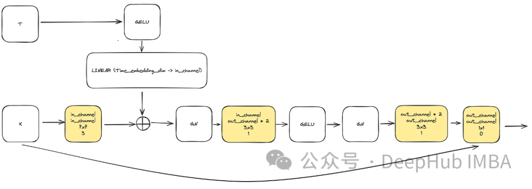
 class ConvNextBlock(nn.Module):
     def __init__(self,
         in_channels,
         out_channels,
         mult=2,
         time_embedding_dim=None,
         norm=True,
         group=8,
     ):
         super().__init__()
         self.mlp = (
             nn.Sequential(nn.GELU(), nn.Linear(time_embedding_dim, in_channels))
             if time_embedding_dim
             else None
         )
 
         self.in_conv = nn.Conv2d(
             in_channels, in_channels, 7, padding=3, groups=in_channels
         )
 
         self.block = nn.Sequential(
             nn.GroupNorm(1, in_channels) if norm else nn.Identity(),
             nn.Conv2d(in_channels, out_channels * mult, 3, padding=1),
             nn.GELU(),
             nn.GroupNorm(1, out_channels * mult),
             nn.Conv2d(out_channels * mult, out_channels, 3, padding=1),
         )
 
         self.residual_conv = (
             nn.Conv2d(in_channels, out_channels, 1)
             if in_channels != out_channels
             else nn.Identity()
         )
 
     def forward(self, x, time_embedding=None):
         h = self.in_conv(x)
         if self.mlp is not None and time_embedding is not None:
             assert self.mlp is not None, "MLP is None"
             h = h + rearrange(self.mlp(time_embedding), "b c -> b c 1 1")
         h = self.block(h)
         return h + self.residual_conv(x)

Sinusoidal Timestamp Embedding

One of the key blocks in the model is the sinusoidal timestamp embedding block, which allows the encoding of a given timestamp to retain information about the current time required for the model’s decoding, as the model will be used for all different timestamps.

This is a very classic implementation and is applied everywhere, so we will directly provide the code.

 class SinusoidalPosEmb(nn.Module):
     def __init__(self, dim, theta=10000):
         super().__init__()
         self.dim = dim
         self.theta = theta
 
     def forward(self, x):
         device = x.device
         half_dim = self.dim // 2
         emb = math.log(self.theta) / (half_dim - 1)
         emb = torch.exp(torch.arange(half_dim, device=device) * -emb)
         emb = x[:, None] * emb[None, :]
         emb = torch.cat((emb.sin(), emb.cos()), dim=-1)
         return emb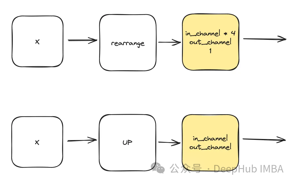

DownSample & UpSample

 class DownSample(nn.Module):
     def __init__(self, dim, dim_out=None):
         super().__init__()
         self.net = nn.Sequential(
             Rearrange("b c (h p1) (w p2) -> b (c p1 p2) h w", p1=2, p2=2),
             nn.Conv2d(dim * 4, default(dim_out, dim), 1),
         )
 
     def forward(self, x):
         return self.net(x)
 
 
 class Upsample(nn.Module):
     def __init__(self, dim, dim_out=None):
         super().__init__()
         self.net = nn.Sequential(
             nn.Upsample(scale_factor=2, mode="nearest"),
             nn.Conv2d(dim, dim_out or dim, kernel_size=3, padding=1),
         )
 
     def forward(self, x):
         return self.net(x)

Temporal Multi-Layer Perceptron

This module utilizes it to create temporal representations based on the given timestamp t. The output of this multi-layer perceptron (MLP) will also serve as input “t” for all modified ConvNext blocks.

Here, “dim” is a hyperparameter of the model that indicates the number of channels required for the first block. It serves as a fundamental calculation for the number of channels in subsequent blocks.

  sinu_pos_emb = SinusoidalPosEmb(dim, theta=10000)
 
   time_dim = dim * 4
 
   time_mlp = nn.Sequential(
       sinu_pos_emb,
       nn.Linear(dim, time_dim),
       nn.GELU(),
       nn.Linear(time_dim, time_dim),
   )

Attention

This is an optional component used in U-Net. Attention helps enhance the role of residual connections in learning. It focuses more on important spatial information obtained from the left side of U-Net through a residual connection calculated by the attention mechanism and feature mappings in the low-dimensional latent space. It originates from the ACC-UNet paper.

The gate represents the upsampling output of the lower block, while x residual represents the residual connection at the level of applying attention.

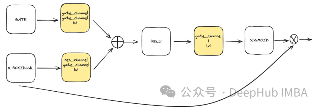
 class BlockAttention(nn.Module):
     def __init__(self, gate_in_channel, residual_in_channel, scale_factor):
         super().__init__()
         self.gate_conv = nn.Conv2d(gate_in_channel, gate_in_channel, kernel_size=1, stride=1)
         self.residual_conv = nn.Conv2d(residual_in_channel, gate_in_channel, kernel_size=1, stride=1)
         self.in_conv = nn.Conv2d(gate_in_channel, 1, kernel_size=1, stride=1)
         self.relu = nn.ReLU()
         self.sigmoid = nn.Sigmoid()
 
     def forward(self, x: torch.Tensor, g: torch.Tensor) -> torch.Tensor:
         in_attention = self.relu(self.gate_conv(g) + self.residual_conv(x))
         in_attention = self.in_conv(in_attention)
         in_attention = self.sigmoid(in_attention)
         return in_attention * x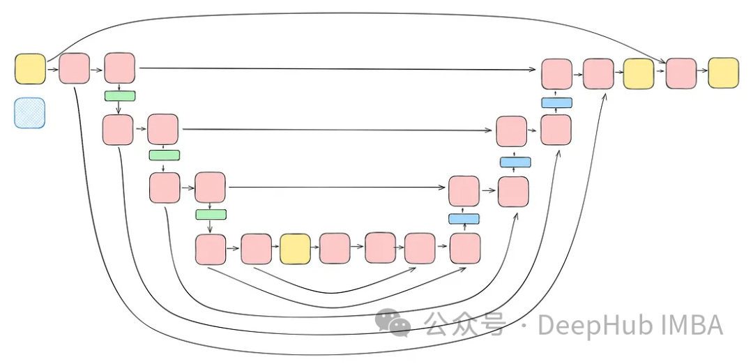

Final Integration

Integrate all the blocks discussed earlier (excluding the attention block) into a U-Net. Each block contains two residual connections instead of one. This modification is made to address potential overfitting issues.

 class DiffusionModel(nn.Module):
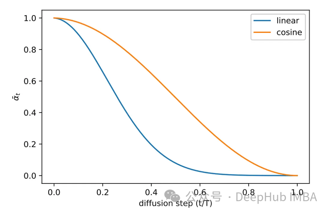
     SCHEDULER_MAPPING = {
         "linear": linear_beta_schedule,
         "cosine": cosine_beta_schedule,
         "sigmoid": sigmoid_beta_schedule,
     }
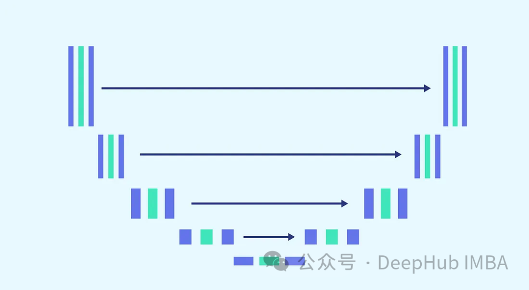
  class TwoResUNet(nn.Module):
     def __init__(self,
         dim,
         init_dim=None,
         out_dim=None,
         dim_mults=(1, 2, 4, 8),
         channels=3,
         sinusoidal_pos_emb_theta=10000,
         convnext_block_groups=8,
     ):
         super().__init__()
         self.channels = channels
         input_channels = channels
         self.init_dim = default(init_dim, dim)
         self.init_conv = nn.Conv2d(input_channels, self.init_dim, 7, padding=3)
 
         dims = [self.init_dim, *map(lambda m: dim * m, dim_mults)]
         in_out = list(zip(dims[:-1], dims[1:]))
 
         sinu_pos_emb = SinusoidalPosEmb(dim, theta=sinusoidal_pos_emb_theta)
 
         time_dim = dim * 4
 
         self.time_mlp = nn.Sequential(
             sinu_pos_emb,
             nn.Linear(dim, time_dim),
             nn.GELU(),
             nn.Linear(time_dim, time_dim),
         )
 
         self.downs = nn.ModuleList([])
         self.ups = nn.ModuleList([])
         num_resolutions = len(in_out)
 
         for ind, (dim_in, dim_out) in enumerate(in_out):
             is_last = ind >= (num_resolutions - 1)
 
             self.downs.append(
                 nn.ModuleList(
                     [
                         ConvNextBlock(
                             in_channels=dim_in,
                             out_channels=dim_in,
                             time_embedding_dim=time_dim,
                             group=convnext_block_groups,
                         ),
                         ConvNextBlock(
                             in_channels=dim_in,
                             out_channels=dim_in,
                             time_embedding_dim=time_dim,
                             group=convnext_block_groups,
                         ),
                         DownSample(dim_in, dim_out)
                         if not is_last
                         else nn.Conv2d(dim_in, dim_out, 3, padding=1),
                     ]
                 )
             )
 
         mid_dim = dims[-1]
         self.mid_block1 = ConvNextBlock(mid_dim, mid_dim, time_embedding_dim=time_dim)
         self.mid_block2 = ConvNextBlock(mid_dim, mid_dim, time_embedding_dim=time_dim)
 
         for ind, (dim_in, dim_out) in enumerate(reversed(in_out)):
             is_last = ind == (len(in_out) - 1)
             is_first = ind == 0
 
             self.ups.append(
                 nn.ModuleList(
                     [
                         ConvNextBlock(
                             in_channels=dim_out + dim_in,
                             out_channels=dim_out,
                             time_embedding_dim=time_dim,
                             group=convnext_block_groups,
                         ),
                         ConvNextBlock(
                             in_channels=dim_out + dim_in,
                             out_channels=dim_out,
                             time_embedding_dim=time_dim,
                             group=convnext_block_groups,
                         ),
                         Upsample(dim_out, dim_in)
                         if not is_last
                         else nn.Conv2d(dim_out, dim_in, 3, padding=1)
                     ]
                 )
             )
 
         default_out_dim = channels
         self.out_dim = default(out_dim, default_out_dim)
 
         self.final_res_block = ConvNextBlock(dim * 2, dim, time_embedding_dim=time_dim)
         self.final_conv = nn.Conv2d(dim, self.out_dim, 1)
 
     def forward(self, x, time):
         b, _, h, w = x.shape
         x = self.init_conv(x)
         r = x.clone()
 
         t = self.time_mlp(time)
 
         unet_stack = []
         for down1, down2, downsample in self.downs:
             x = down1(x, t)
             unet_stack.append(x)
             x = down2(x, t)
             unet_stack.append(x)
             x = downsample(x)
 
         x = self.mid_block1(x, t)
         x = self.mid_block2(x, t)
 
         for up1, up2, upsample in self.ups:
             x = torch.cat((x, unet_stack.pop()), dim=1)
             x = up1(x, t)
             x = torch.cat((x, unet_stack.pop()), dim=1)
             x = up2(x, t)
             x = upsample(x)
 
         x = torch.cat((x, r), dim=1)
         x = self.final_res_block(x, t)
 
         return self.final_conv(x) class TwoResUNet(nn.Module):
     def __init__(
         self,
         model: nn.Module,
         image_size: int,
         *,
         beta_scheduler: str = "linear",
         timesteps: int = 1000,
         schedule_fn_kwargs: dict | None = None,
         auto_normalize: bool = True,
     ) -> None:
         super().__init__()
         self.model = model
 
         self.channels = self.model.channels
         self.image_size = image_size
 
         self.beta_scheduler_fn = self.SCHEDULER_MAPPING.get(beta_scheduler)
         if self.beta_scheduler_fn is None:
             raise ValueError(f"unknown beta schedule {beta_scheduler}")
 
         if schedule_fn_kwargs is None:
             schedule_fn_kwargs = {}
 
         betas = self.beta_scheduler_fn(timesteps, **schedule_fn_kwargs)
         alphas = 1.0 - betas
         alphas_cumprod = torch.cumprod(alphas, dim=0)
         alphas_cumprod_prev = F.pad(alphas_cumprod[:-1], (1, 0), value=1.0)
         posterior_variance = (
             betas * (1.0 - alphas_cumprod_prev) / (1.0 - alphas_cumprod)
         )
 
         register_buffer = lambda name, val: self.register_buffer(
             name, val.to(torch.float32)
         )
 
         register_buffer("betas", betas)
         register_buffer("alphas_cumprod", alphas_cumprod)
         register_buffer("alphas_cumprod_prev", alphas_cumprod_prev)
         register_buffer("sqrt_recip_alphas", torch.sqrt(1.0 / alphas))
         register_buffer("sqrt_alphas_cumprod", torch.sqrt(alphas_cumprod))
         register_buffer(
             "sqrt_one_minus_alphas_cumprod", torch.sqrt(1.0 - alphas_cumprod)
         )
         register_buffer("posterior_variance", posterior_variance)
 
         timesteps, *_ = betas.shape
         self.num_timesteps = int(timesteps)
 
         self.sampling_timesteps = timesteps
 
         self.normalize = normalize_to_neg_one_to_one if auto_normalize else identity
         self.unnormalize = unnormalize_to_zero_to_one if auto_normalize else identity
 
     @torch.inference_mode()
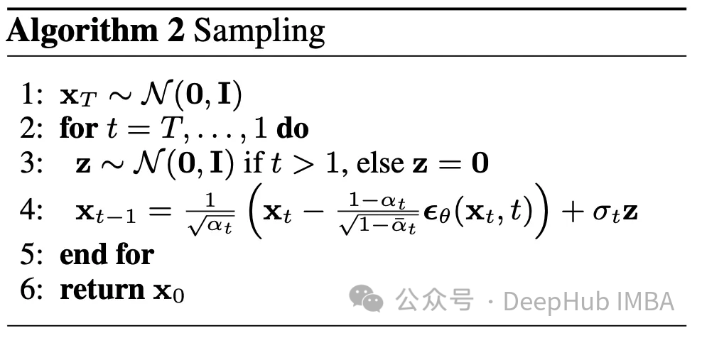
     def p_sample(self, x: torch.Tensor, timestamp: int) -> torch.Tensor:
         b, *_, device = *x.shape, x.device
         batched_timestamps = torch.full(
             (b,), timestamp, device=device, dtype=torch.long
         )
 
         preds = self.model(x, batched_timestamps)
 
         betas_t = extract(self.betas, batched_timestamps, x.shape)
         sqrt_recip_alphas_t = extract(
             self.sqrt_recip_alphas, batched_timestamps, x.shape
         )
         sqrt_one_minus_alphas_cumprod_t = extract(
             self.sqrt_one_minus_alphas_cumprod, batched_timestamps, x.shape
         )
 
         predicted_mean = sqrt_recip_alphas_t * (
             x - betas_t * preds / sqrt_one_minus_alphas_cumprod_t
         )
 
         if timestamp == 0:
             return predicted_mean
         else:
             posterior_variance = extract(
                 self.posterior_variance, batched_timestamps, x.shape
             )
             noise = torch.randn_like(x)
             return predicted_mean + torch.sqrt(posterior_variance) * noise
 
     @torch.inference_mode()
     def p_sample_loop(
         self, shape: tuple, return_all_timesteps: bool = False
     ) -> torch.Tensor:
         batch, device = shape[0], "mps"
 
         img = torch.randn(shape, device=device)
         # This cause me a RunTimeError on MPS device due to MPS back out of memory
         # No ideas how to resolve it at this point
 
         # imgs = [img]
 
         for t in tqdm(reversed(range(0, self.num_timesteps)), total=self.num_timesteps):
             img = self.p_sample(img, t)
             # imgs.append(img)
 
         ret = img  # if not return_all_timesteps else torch.stack(imgs, dim=1)
 
         ret = self.unnormalize(ret)
         return ret
 
     def sample(
         self, batch_size: int = 16, return_all_timesteps: bool = False
     ) -> torch.Tensor:
         shape = (batch_size, self.channels, self.image_size, self.image_size)
         return self.p_sample_loop(shape, return_all_timesteps=return_all_timesteps)
 
     def q_sample(
         self, x_start: torch.Tensor, t: int, noise: torch.Tensor = None
     ) -> torch.Tensor:
         if noise is None:
             noise = torch.randn_like(x_start)
 
         sqrt_alphas_cumprod_t = extract(self.sqrt_alphas_cumprod, t, x_start.shape)
         sqrt_one_minus_alphas_cumprod_t = extract(
             self.sqrt_one_minus_alphas_cumprod, t, x_start.shape
         )
 
         return sqrt_alphas_cumprod_t * x_start + sqrt_one_minus_alphas_cumprod_t * noise
 
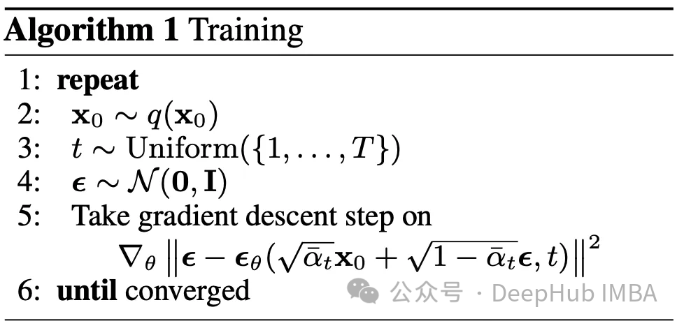
     def p_loss(
         self,
         x_start: torch.Tensor,
         t: int,
         noise: torch.Tensor = None,
         loss_type: str = "l2",
     ) -> torch.Tensor:
         if noise is None:
             noise = torch.randn_like(x_start)
         x_noised = self.q_sample(x_start, t, noise=noise)
         predicted_noise = self.model(x_noised, t)
 
         if loss_type == "l2":
             loss = F.mse_loss(noise, predicted_noise)
         elif loss_type == "l1":
             loss = F.l1_loss(noise, predicted_noise)
         else:
             raise ValueError(f"unknown loss type {loss_type}")
         return loss
 
     def forward(self, x: torch.Tensor) -> torch.Tensor:
         b, c, h, w, device, img_size = *x.shape, x.device, self.image_size
         assert h == w == img_size, f"image size must be {img_size}"
 
         timestamp = torch.randint(0, self.num_timesteps, (1,)).long().to(device)
         x = self.normalize(x)
         return self.p_loss(x, timestamp)

Implementation of Diffusion

Finally, we introduce how diffusion is implemented. Since we have already covered all the mathematical theories used in the forward, reverse, and sampling processes, we will focus on the code here.

 class DiffusionModel(nn.Module):
     SCHEDULER_MAPPING = {
         "linear": linear_beta_schedule,
         "cosine": cosine_beta_schedule,
         "sigmoid": sigmoid_beta_schedule,
     }
 
     def __init__(
         self,
         model: nn.Module,
         image_size: int,
         *,
         beta_scheduler: str = "linear",
         timesteps: int = 1000,
         schedule_fn_kwargs: dict | None = None,
         auto_normalize: bool = True,
     ) -> None:
         super().__init__()
         self.model = model
 
         self.channels = self.model.channels
         self.image_size = image_size
 
         self.beta_scheduler_fn = self.SCHEDULER_MAPPING.get(beta_scheduler)
         if self.beta_scheduler_fn is None:
             raise ValueError(f"unknown beta schedule {beta_scheduler}")
 
         if schedule_fn_kwargs is None:
             schedule_fn_kwargs = {}
 
         betas = self.beta_scheduler_fn(timesteps, **schedule_fn_kwargs)
         alphas = 1.0 - betas
         alphas_cumprod = torch.cumprod(alphas, dim=0)
         alphas_cumprod_prev = F.pad(alphas_cumprod[:-1], (1, 0), value=1.0)
         posterior_variance = (
             betas * (1.0 - alphas_cumprod_prev) / (1.0 - alphas_cumprod)
         )
 
         register_buffer = lambda name, val: self.register_buffer(
             name, val.to(torch.float32)
         )
 
         register_buffer("betas", betas)
         register_buffer("alphas_cumprod", alphas_cumprod)
         register_buffer("alphas_cumprod_prev", alphas_cumprod_prev)
         register_buffer("sqrt_recip_alphas", torch.sqrt(1.0 / alphas))
         register_buffer("sqrt_alphas_cumprod", torch.sqrt(alphas_cumprod))
         register_buffer(
             "sqrt_one_minus_alphas_cumprod", torch.sqrt(1.0 - alphas_cumprod)
         )
         register_buffer("posterior_variance", posterior_variance)
 
         timesteps, *_ = betas.shape
         self.num_timesteps = int(timesteps)
 
         self.sampling_timesteps = timesteps
 
         self.normalize = normalize_to_neg_one_to_one if auto_normalize else identity
         self.unnormalize = unnormalize_to_zero_to_one if auto_normalize else identity
 
     @torch.inference_mode()
     def p_sample(self, x: torch.Tensor, timestamp: int) -> torch.Tensor:
         b, *_, device = *x.shape, x.device
         batched_timestamps = torch.full(
             (b,), timestamp, device=device, dtype=torch.long
         )
 
         preds = self.model(x, batched_timestamps)
 
         betas_t = extract(self.betas, batched_timestamps, x.shape)
         sqrt_recip_alphas_t = extract(
             self.sqrt_recip_alphas, batched_timestamps, x.shape
         )
         sqrt_one_minus_alphas_cumprod_t = extract(
             self.sqrt_one_minus_alphas_cumprod, batched_timestamps, x.shape
         )
 
         predicted_mean = sqrt_recip_alphas_t * (
             x - betas_t * preds / sqrt_one_minus_alphas_cumprod_t
         )
 
         if timestamp == 0:
             return predicted_mean
         else:
             posterior_variance = extract(
                 self.posterior_variance, batched_timestamps, x.shape
             )
             noise = torch.randn_like(x)
             return predicted_mean + torch.sqrt(posterior_variance) * noise
 
     @torch.inference_mode()
     def p_sample_loop(
         self, shape: tuple, return_all_timesteps: bool = False
     ) -> torch.Tensor:
         batch, device = shape[0], "mps"
 
         img = torch.randn(shape, device=device)
         # This cause me a RunTimeError on MPS device due to MPS back out of memory
         # No ideas how to resolve it at this point
 
         # imgs = [img]
 
         for t in tqdm(reversed(range(0, self.num_timesteps)), total=self.num_timesteps):
             img = self.p_sample(img, t)
             # imgs.append(img)
 
         ret = img  # if not return_all_timesteps else torch.stack(imgs, dim=1)
 
         ret = self.unnormalize(ret)
         return ret
 
     def sample(
         self, batch_size: int = 16, return_all_timesteps: bool = False
     ) -> torch.Tensor:
         shape = (batch_size, self.channels, self.image_size, self.image_size)
         return self.p_sample_loop(shape, return_all_timesteps=return_all_timesteps)
 
     def q_sample(
         self, x_start: torch.Tensor, t: int, noise: torch.Tensor = None
     ) -> torch.Tensor:
         if noise is None:
             noise = torch.randn_like(x_start)
 
         sqrt_alphas_cumprod_t = extract(self.sqrt_alphas_cumprod, t, x_start.shape)
         sqrt_one_minus_alphas_cumprod_t = extract(
             self.sqrt_one_minus_alphas_cumprod, t, x_start.shape
         )
 
         return sqrt_alphas_cumprod_t * x_start + sqrt_one_minus_alphas_cumprod_t * noise
 
     def p_loss(
         self,
         x_start: torch.Tensor,
         t: int,
         noise: torch.Tensor = None,
         loss_type: str = "l2",
     ) -> torch.Tensor:
         if noise is None:
             noise = torch.randn_like(x_start)
         x_noised = self.q_sample(x_start, t, noise=noise)
         predicted_noise = self.model(x_noised, t)
 
         if loss_type == "l2":
             loss = F.mse_loss(noise, predicted_noise)
         elif loss_type == "l1":
             loss = F.l1_loss(noise, predicted_noise)
         else:
             raise ValueError(f"unknown loss type {loss_type}")
         return loss
 
     def forward(self, x: torch.Tensor) -> torch.Tensor:
         b, c, h, w, device, img_size = *x.shape, x.device, self.image_size
         assert h == w == img_size, f"image size must be {img_size}"
 
         timestamp = torch.randint(0, self.num_timesteps, (1,)).long().to(device)
         x = self.normalize(x)
         return self.p_loss(x, timestamp)

Summary of Training Points

For the training phase, we set up 37,000 training steps with a batch size of 16. Due to GPU memory allocation limits, the image size is restricted to 128×128. Using exponential moving average (EMA) model weights, samples are generated every 1000 steps to smooth sampling and save model versions.

In the initial 1000 training steps, the model began to capture some features but still missed certain areas. Around 10,000 steps, the model began to produce promising results, and progress became more apparent. By the end of 30,000 steps, the quality of the results improved significantly, but there were still black images. This was simply because the model did not have enough sample variety, and the data distribution of real images did not fully map to the Gaussian distribution.

With the final model weights, we can generate some images. Although the image quality is limited due to the 128×128 size restriction, the performance of the model is still commendable.

Note: The dataset used in this article consists of satellite images of forest terrain; please refer to the ETL section in the source code for specific acquisition methods.

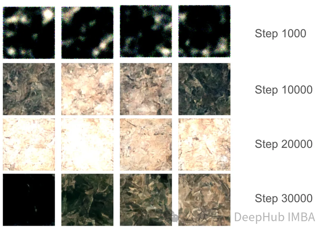
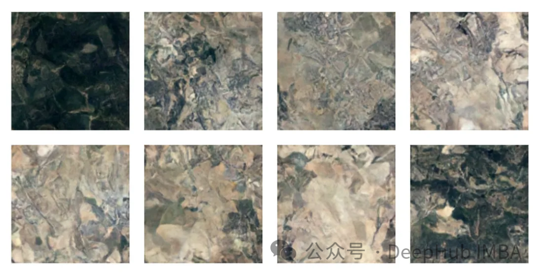
Conclusion

We have comprehensively introduced the necessary knowledge about diffusion models and have implemented them completely using PyTorch.

The code for this article:

https://github.com/Camaltra/this-is-not-real-aerial-imagery/

About Us

MLNLP Community is a grassroots academic community jointly established by domestic and foreign scholars in machine learning and natural language processing. It has now developed into a well-known community for machine learning and natural language processing in China and abroad, aiming to promote progress between the academic and industrial circles of machine learning and natural language processing and enthusiasts.

The community can provide an open communication platform for related practitioners in further studies, employment, and research. Everyone is welcome to follow and join us.