Introduction to RNN and ODE: Understanding RNNs

Author: Su Jianlin

Affiliation: Guangzhou Flame Information Technology Co., Ltd.

Research Direction: NLP, Neural Networks

Personal Homepage: kexue.fm

I had originally decided to stop working with RNNs as they actually correspond to numerical methods for ODEs (Ordinary Differential Equations). This realization provided me with insights into something I have always wanted to do—using deep learning to solve some pure mathematical problems. In fact, this is quite an interesting and useful result, so I would like to introduce it. Additionally, this article also involves writing your own RNN, so it can also serve as a simple tutorial for creating custom RNN layers.

Note: This article is not an introduction to the recent hot topic of “Neural ODEs” [1], but it has some connections.

Basics of RNN

What is RNN?

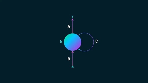
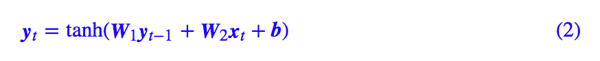
As we all know, RNN stands for “Recurrent Neural Network”, which, unlike CNN, can be considered a general term for a class of models rather than a single model. Simply put, any model that takes a sequence of input vectors (x1,x2,…,xT) and outputs another sequence of vectors (y1,y2,…,yT), satisfying the following recursive relationship, can be called RNN.

Introduction to RNN and ODE: Understanding RNNs

Because of this, the original simple RNN, as well as improved models like GRU, LSTM, and SRU, are all referred to as RNNs, as they can all be seen as special cases of the above formula. Some topics that seem unrelated to RNN, such as the denominator calculation of CRF introduced recently, are actually also a simple RNN.

In short, RNN is essentially recursive computation.

Writing Your Own RNN

Here we will first introduce how to quickly and easily write a custom RNN using Keras.

In fact, whether in Keras or pure TensorFlow, customizing your own RNN is not complicated. In Keras, you just need to write the recursive function for each step; while in TensorFlow, it is slightly more complex, as you need to encapsulate each step’s recursive function into an RNNCell class.

Below is the implementation of the most basic RNN using Keras:

Introduction to RNN and ODE: Understanding RNNs

The code is very simple:

#! -*- coding: utf-8- -*-

from keras.layers import Layer
import keras.backend as K


class My_RNN(Layer):

    def __init__(self, output_dim, **kwargs):
        self.output_dim = output_dim # Output dimension
        super(My_RNN, self).__init__(**kwargs)

    def build(self, input_shape): # Define trainable parameters
        self.kernel1 = self.add_weight(name='kernel1',
                                      shape=(self.output_dim, self.output_dim),
                                      initializer='glorot_normal',
                                      trainable=True)
        self.kernel2 = self.add_weight(name='kernel2',
                                      shape=(input_shape[-1], self.output_dim),
                                      initializer='glorot_normal',
                                      trainable=True)
        self.bias = self.add_weight(name='kernel',
                                      shape=(self.output_dim,),
                                      initializer='glorot_normal',
                                      trainable=True)

    def step_do(self, step_in, states): # Define each step's iteration
        step_out = K.tanh(K.dot(states[0], self.kernel1) +
                          K.dot(step_in, self.kernel2) +
                          self.bias)
        return step_out, [step_out]

    def call(self, inputs): # Define the function for execution
        init_states = [K.zeros((K.shape(inputs)[0],
                                self.output_dim)
                              )] # Define initial state (all zeros)
        outputs = K.rnn(self.step_do, inputs, init_states) # Loop through step_do function
        return outputs[0] # outputs is a tuple, outputs[0] is the last output,
                          # outputs[1] is the entire output sequence,
                          # outputs[2] is a list,
                          # which contains intermediate hidden states.

    def compute_output_shape(self, input_shape):
        return (input_shape[0], self.output_dim)

As you can see, while there are quite a few lines of code, most of them are just fixed format statements, the real definition of RNN lies in the step_do function. This function takes two inputs: step_in and states. Here, step_in is a tensor of shape (batch_size, input_dim) representing the current sample xt, while states is a list representing yt−1 and some intermediate variables.

It is particularly important to note that states is a list of tensors, not a single tensor, because multiple intermediate variables may need to be passed simultaneously during the recursion, not just yt−1. For example, LSTM requires two state tensors. Finally, step_do must return yt and the new states, which is the specification for writing this step’s function.

The K.rnn function accepts three basic parameters (there are other parameters, please refer to the official documentation), where the first parameter is the step_do function we just wrote, the second parameter is the input time series, and the third is the initial state, which is consistent with the states mentioned earlier. Therefore, it is natural that init_states is also a list of tensors, and by default, we will choose to initialize it to all zeros.

Basics of ODE

What is ODE?

ODE stands for “Ordinary Differential Equation”, referring to a general system of ordinary differential equations:

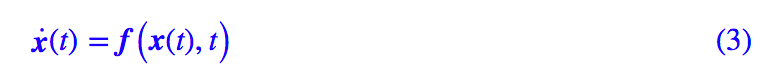
Introduction to RNN and ODE: Understanding RNNs

The field of ODE research is often directly referred to as “dynamics” or “dynamical systems”, because Newtonian mechanics is typically just a set of ODEs.

ODEs can produce a rich variety of functions. For example, e^t is actually the solution to x˙=x, and sint and cost are both solutions to x¨+x=0 (with different initial conditions). In fact, I remember that there are indeed some tutorials that directly define the e^t function through the differential equation x˙=x. Besides these elementary functions, many special functions that we can name but do not know what they are, are derived from ODEs, such as hypergeometric functions, Legendre functions, Bessel functions…

In short, ODE can produce and has produced all sorts of strange functions.

Numerical Solutions for ODE

It is actually very rare to find ODEs that can be solved analytically, so most of the time we need numerical methods.

The numerical solution of ODE is already a very mature discipline, and here we will not go into much detail, just introduce the most basic iterative formula proposed by the mathematician Euler:

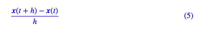
Introduction to RNN and ODE: Understanding RNNs

Here, h is the step size. Euler’s method is quite simple, as it uses:

Introduction to RNN and ODE: Understanding RNNs

to approximate the derivative term x˙(t). As long as the initial condition x(0) is given, we can iteratively calculate the results at each time point based on (4).

ODE and RNN

ODE is also RNN

Can you find any connection by carefully comparing (4) and (1)?

In (1), t is an integer variable, while in (4), t is a floating-point variable. Other than that, there seems to be no obvious difference between (4) and (1). In fact, in (4), we can treat h as the time unit, setting t=nh, then (4) becomes:

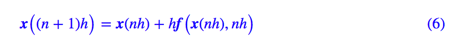
Introduction to RNN and ODE: Understanding RNNs

Now, we can see that the time variable n in (6) is also an integer. Thus, we know that Euler’s method for ODE (4) is actually a special case of RNN. This may help us indirectly understand why RNN has such strong fitting capabilities, especially for time series data. We see that ODE can produce many complex functions, and since ODE is merely a special case of RNN, RNN can also produce more complex functions.

Using RNN to Solve ODE

Thus, we can write an RNN to solve ODE, for example, in the case of the “Two Species Competition Model”[2]:

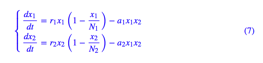
Introduction to RNN and ODE: Understanding RNNs

We can write:

#! -*- coding: utf-8- -*-

from keras.layers import Layer
import keras.backend as K


class ODE_RNN(Layer):

    def __init__(self, steps, h, **kwargs):
        self.steps = steps
        self.h = h
        super(ODE_RNN, self).__init__(**kwargs)

    def step_do(self, step_in, states): # Define each step's iteration
        x = states[0]
        r1,r2,a1,a2,iN1,iN2 = 0.1,0.3,0.0001,0.0002,0.002,0.003
        _1 = r1 * x[:,0] * (1 - iN1 * x[:,0]) - a1 * x[:,0] * x[:,1]
        _2 = r2 * x[:,1] * (1 - iN2 * x[:,1]) - a2 * x[:,0] * x[:,1]
        _1 = K.expand_dims(_1, 1)
        _2 = K.expand_dims(_2, 1)
        _ = K.concatenate([_1, _2], 1)
        step_out = x + self.h * _
        return step_out, [step_out]

    def call(self, inputs): # Here, inputs are the initial conditions
        init_states = [inputs]
        zeros = K.zeros((K.shape(inputs)[0],
                         self.steps,
                         K.shape(inputs)[1])) # The iterative process does not require external input, so
                                              # we specify a zero input just for formal passing
        outputs = K.rnn(self.step_do, zeros, init_states) # Loop through step_do function
        return outputs[1] # This time we output the entire result sequence

    def compute_output_shape(self, input_shape):
        return (input_shape[0], self.steps, input_shape[1])


from keras.models import Sequential
import numpy as np
import matplotlib.pyplot as plt


steps,h = 1000,0.1

M = Sequential()
M.add(ODE_RNN(steps, h, input_shape=(2,)))
M.summary()

# Direct forward propagation outputs the solution
result = M.predict(np.array([[100, 150]]))[0] # Calculate using [100, 150] as the initial condition
times = np.arange(1, steps+1) * h

# Plotting
plt.plot(times, result[:,0])
plt.plot(times, result[:,1])
plt.savefig('test.png')

The entire process is easy to understand, but there are two points to note. First, as the system of equations (7) is only two-dimensional and not easy to express in matrix operations, I directly operated element-wise in the step_do function (x[:,0],x[:,1]). If the equations themselves have a higher dimension and can be expressed in matrix operations, it would be more efficient to write it using matrix operations. Secondly, after writing the entire model, we can directly use predict to output results without needing to “train”.

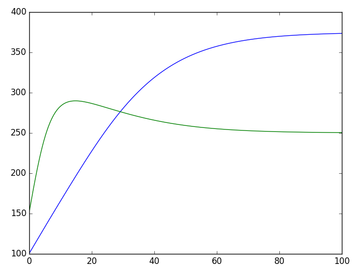
Introduction to RNN and ODE: Understanding RNNs

▲ RNN solving the two species competition model

Inferring ODE Parameters

The previous section’s introduction indicates that the forward propagation of RNN corresponds to Euler’s method for ODE, so what does backward propagation correspond to?

In practical problems, there is a class of problems called “model inference”, which is about guessing the model (mechanism inference) that fits a batch of experimental data. This typically involves two steps: first, guessing the form of the model, and second, determining the parameters of the model. Assuming that this batch of data can be described by an ODE and the form of this ODE is already known, we then need to estimate the parameters within.

If the ODE can be completely solved analytically, then it is just a very simple regression problem. However, as previously mentioned, most ODEs do not have analytical solutions, so numerical methods become necessary. This is essentially what the backward propagation of ODE corresponds to in RNN: forward propagation is solving the ODE (the prediction process of RNN), and backward propagation is naturally inferring the parameters of the ODE (the training process of RNN). This is a very interesting fact: parameter inference for ODE is a well-researched topic, yet in deep learning, it is merely a basic application of RNN.

We can save the solution data from the previous example of the differential equation, then take a few points to see if we can infer the original differential equation. The solution data is as follows:

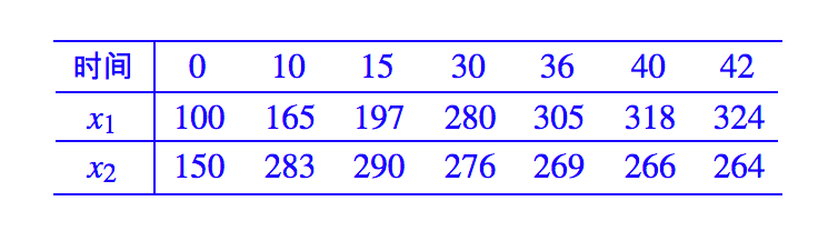
Introduction to RNN and ODE: Understanding RNNs

Assuming we only know this limited point data, we can then assume the form of equation (7) and estimate the parameters of the equation. Let’s modify the previous code:

#! -*- coding: utf-8- -*-

from keras.layers import Layer
import keras.backend as K


def my_init(shape, dtype=None): # Initialization needs to be defined, which is equivalent to estimating the magnitude of parameters
    return K.variable([0.1, 0.1, 0.001, 0.001, 0.001, 0.001])


class ODE_RNN(Layer):

    def __init__(self, steps, h, **kwargs):
        self.steps = steps
        self.h = h
        super(ODE_RNN, self).__init__(**kwargs)

    def build(self, input_shape): # Make the original parameters trainable
        self.kernel = self.add_weight(name='kernel', 
                                      shape=(6,),
                                      initializer=my_init,
                                      trainable=True)
    def step_do(self, step_in, states): # Define each step's iteration
        x = states[0]
        r1,r2,a1,a2,iN1,iN2 = (self.kernel[0], self.kernel[1],
                               self.kernel[2], self.kernel[3],
                               self.kernel[4], self.kernel[5])
        _1 = r1 * x[:,0] * (1 - iN1 * x[:,0]) - a1 * x[:,0] * x[:,1]
        _2 = r2 * x[:,1] * (1 - iN2 * x[:,1]) - a2 * x[:,0] * x[:,1]
        _1 = K.expand_dims(_1, 1)
        _2 = K.expand_dims(_2, 1)
        _ = K.concatenate([_1, _2], 1)
        step_out = x + self.h * K.clip(_, -1e5, 1e5) # Prevent gradient explosion
        return step_out, [step_out]

    def call(self, inputs): # Here, inputs are the initial conditions
        init_states = [inputs]
        zeros = K.zeros((K.shape(inputs)[0],
                         self.steps,
                         K.shape(inputs)[1])) # The iterative process does not require external input, so
                                              # we specify a zero input just for formal passing
        outputs = K.rnn(self.step_do, zeros, init_states) # Loop through step_do function
        return outputs[1] # This time we output the entire result sequence

    def compute_output_shape(self, input_shape):
        return (input_shape[0], self.steps, input_shape[1])


from keras.models import Sequential
from keras.optimizers import Adam
import numpy as np
import matplotlib.pyplot as plt


steps,h = 50, 1 # Use a large step size to reduce the number of steps, weaken long-term dependencies, and speed up inference
series = {0: [100, 150],
          10: [165, 283],
          15: [197, 290],
          30: [280, 276],
          36: [305, 269],
          40: [318, 266],
          42: [324, 264]}

M = Sequential()
M.add(ODE_RNN(steps, h, input_shape=(2,)))
M.summary()

# Build training samples
# There is actually only one sample sequence, X is the initial condition, Y is the subsequent time series
X = np.array([series[0]])
Y = np.zeros((1, steps, 2))

for i,j in series.items():
    if i != 0:
        Y[0, int(i/h)-1] += series[i]

# Custom loss
# When training, only consider the moments with data, the moments without data are ignored
def ode_loss(y_true, y_pred):
    T = K.sum(K.abs(y_true), 2, keepdims=True)
    T = K.cast(K.greater(T, 1e-3), 'float32')
    return K.sum(T * K.square(y_true - y_pred), [1, 2])

M.compile(loss=ode_loss,
          optimizer=Adam(1e-4))

M.fit(X, Y, epochs=10000) # Train for enough epochs with a low learning rate

# Use the trained model to predict again, plot, and compare results
result = M.predict(np.array([[100, 150]]))[0]
times = np.arange(1, steps+1) * h

plt.clf()
plt.plot(times, result[:,0], color='blue')
plt.plot(times, result[:,1], color='green')
plt.plot(series.keys(), [i[0] for i in series.values()], 'o', color='blue')
plt.plot(series.keys(), [i[1] for i in series.values()], 'o', color='green')
plt.savefig('test.png')

The results can be viewed in one chart:

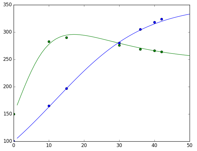
Introduction to RNN and ODE: Understanding RNNs

▲ RNN’s parameter estimation effect for ODE

(Scatter points: limited experimental data, curves: estimated model)

Clearly, the results are satisfactory.

Conclusion

This article introduced the RNN model and its custom implementation in Keras within a general framework, and revealed the connection between ODE and RNN. Based on this, it discussed the basic ideas of using RNN to directly solve ODEs and inferring ODE parameters using RNN.

Readers are reminded that in the backward propagation of RNN models, careful initialization and truncation handling should be done, and learning rates should be chosen properly to prevent gradient explosion (gradient vanishing is just a matter of insufficient optimization, while gradient explosion leads to a complete crash, making resolving gradient explosion particularly important).

In summary, gradient vanishing and explosion are classic difficulties in RNNs. In fact, the introduction of models like LSTM and GRU fundamentally aims to solve the gradient vanishing problem of RNNs, while gradient explosion is addressed by using tanh or sigmoid activation functions.

However, when solving ODEs with RNNs, we have no choice over the activation function (the activation function is part of the ODE), so we can only carefully handle initialization and other factors. It is said that as long as careful initialization is done, using relu as the activation function in ordinary RNNs is not a problem.

Introduction to RNN and ODE: Understanding RNNs

Basics of RNN

Basics of ODE

ODE and RNN

Conclusion

Related Links

Leave a Comment Cancel reply