
Editorial Department
WeChat Official Account
KeywordsSearch across the webLatest Ranking
『Quantitative Investment』: Ranked First
『Quantitative』: Ranked First
『Machine Learning』: Ranked Third
We will continue to work hard
To become a qualityfinancial and technical public account across the web
Today we will read an article from Guosen Securities Research
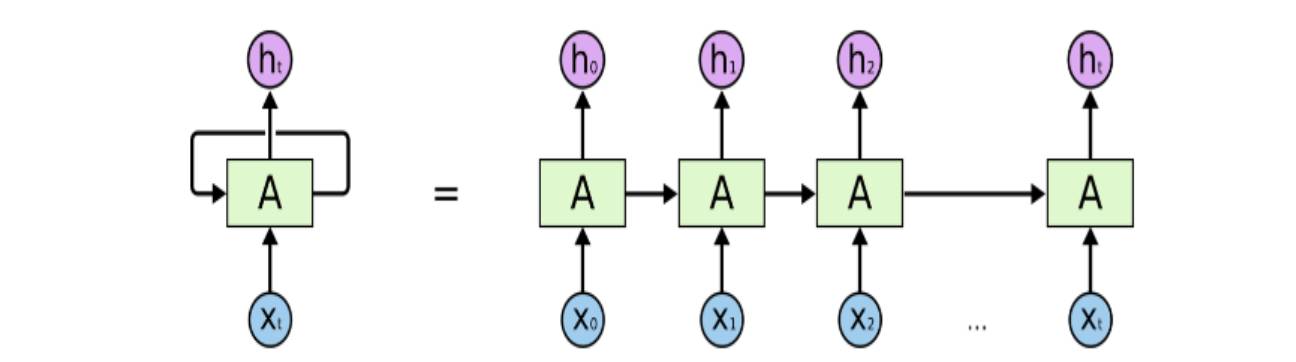
Introduction to RNN
The biggest feature that distinguishes RNN from traditional neural networks, such as perceptrons, is its connection to time. It includes a recurrent network where the output at the next time step is influenced not only by the input at that time but also by the output from the previous time step. This means that information has a lasting impact. In practical terms, this is easy to understand; when people see new information, their views or judgments are not solely responses to the current information but also involve prior experiences and thoughts. The human brain is not a blank slate; it contains many prior pieces of information, indicating the existence and persistence of thought. For example, if you want to classify the types of events occurring at various points in a movie as warm, romantic, violent, etc., it is quite difficult to achieve this using traditional neural networks. However, RNNs, with their memory capabilities, can handle this problem well.
LSTM Stock Selection Model
When predicting information that is far apart, the efficiency of the original RNN structure is not satisfactory. Although some scholars have proven that we can achieve the goal of predicting distant information by carefully designing parameters, this is undoubtedly costly and difficult to implement, thus losing practical significance.
LSTM (Long-Short Term Memory) networks were created to solve the long-term dependency problem mentioned above. LSTM is a carefully designed RNN network. Although LSTM and the original RNN both have three main layers—input layer, hidden layer, and output layer—there are significant differences in the design of the hidden layer. The main difference is that LSTM has a special cell structure in the hidden layer.
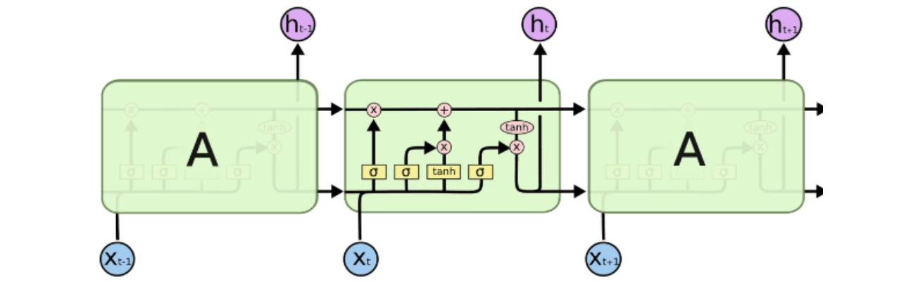
LSTM changes a simple activation into a storage unit cell that is a linear combination of several parts. This allows for controlling the output information for the next step, such as whether to include previous information and how much to include. It is akin to receiving reminders about important information before proceeding with the next operation.
Parameter Settings
Backtesting Period: May 1, 2007 – April 30, 2016, with over 180,000 monthly data training samples during this period (each stock at the end of each month represents one sample).
Strategy Period: May 1, 2016 – April 30, 2017
RNN Time Length (steps): 24 months, meaning each training sample includes factor data from the past 24 months, sequentially inputting from the first month into the neural network, and simultaneously looping the return value with the next month’s factor into the neural network, continuing until obtaining the prediction value for the 24th month.
Number of Factors: Since we do not evaluate the effectiveness of factors at the beginning of training in the neural network, we also do not merge factors, inputting all into the model (excluding some factors with excessive correlation that belong to the same category, which can reduce the likelihood of overfitting in model training). Ultimately, 48 small factors were selected, belonging to 10 common style factors.
Number of Classes: To verify the accuracy of predictions and exclude some noise from the samples, we divided the sample return types into three categories: Up (monthly return greater than 3%), Down (monthly return less than -3%), and Neutral (monthly return between -3% and 3%).
Enhancements to RNN
From the parameter settings of the original model and the characteristics of deep learning algorithms, we can easily categorize enhancements to neural networks into two routes: improvements in data structure and enhancements to neural network algorithms.
Data Improvements
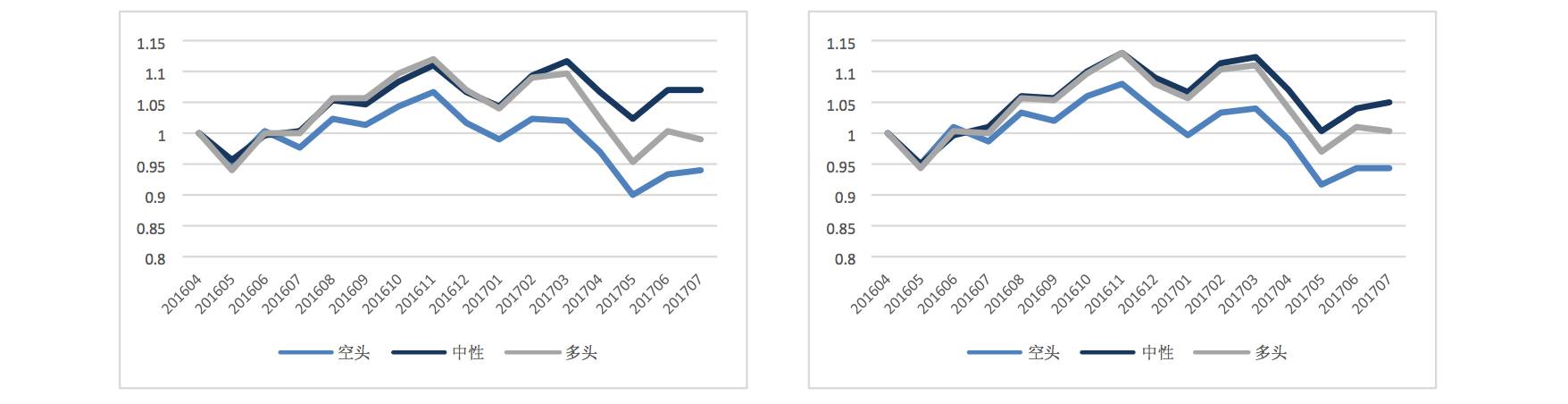
1. Relative vs. Absolute Returns: In the original model, we used the absolute value of the next period’s stock return of 3% as the label for the sample. However, categorizing historical samples by absolute value leads to inconsistent sample quantities across different periods. Therefore, we tried using relative returns for sample categorization. Specifically, we considered dividing each period’s return into the top 30% (bullish), bottom 30% (bearish), and middle 40% (neutral) based on the number of stocks.
Absolute Return Labels | Relative Return Labels
It can be observed that relative returns yield more significant results compared to absolute return label structures, although the final return rate differences are not substantial. The neutral combination still cannot be distinguished from the bullish combination.
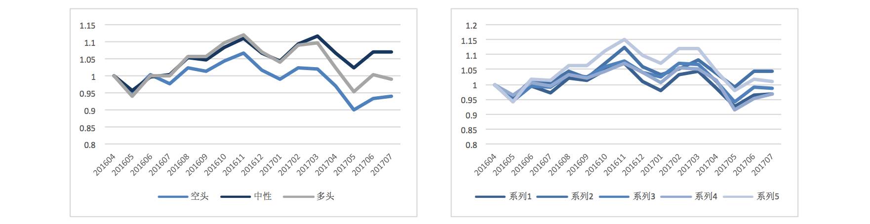
2. The second data processing consideration is the number of input features. In the previous report, we selected 48 small factors as input data features, which included the traditional 10 major factor styles. Due to multicollinearity issues among factors, using 48 factors is relatively excessive and contains a lot of collinearity information. In this processing, I considered selecting only representative style factors, ultimately choosing 12 factors including PE, cash flow volatility, revenue growth rate, net profit growth rate, book value leverage, one-month turnover, one-month momentum, market capitalization, BP, price logarithm, BETA, and ROE.
48 Input Features | 48 Input Features
3. Since RNN neural networks require each input sample to include its historical feature sequence, in the previous report, we used the past 24 months as input features. This time, we shortened the historical length to 12 months; however, the actual difference was not significant.
24 Months RNN | 24 Months RNN
4. Finally, we attempted to improve the prediction accuracy of the neural network by increasing the number of classifications from 3 to 5: over 5%, 3%-5%, -3%-3%, -3%-5%, and a drop of over -5%.
3-Class Division | 5-Class Division
From the results, the 5-class effect was poorer, and the prediction of the highest increase was not significant.
In summary, improvements made to the model from the data input side have not achieved effective enhancements, especially the predictions of neutral categories often fail.
Algorithm Improvements
Another enhancement approach for RNN focuses on improving the learning algorithm. This time, we will introduce a relatively mainstream RNN neural network extension: Adaptive Computation Time (ACT).
RNN-ACT
From the characteristics of deep neural networks, increasing the depth of the network can empirically enhance learning effectiveness. However, based on the algorithm characteristics of RNN, with an increase in layers, RNN networks using tanh as the activation function face the problem of vanishing gradients.
ACT proposes an alternative direction for increasing depth, which is to increase the number of repetitions of learning the same batch of data during each learning iteration, thereby enhancing the complexity of the RNN network.
A complete structure of an ACT recursive neural network is shown in the figure below:
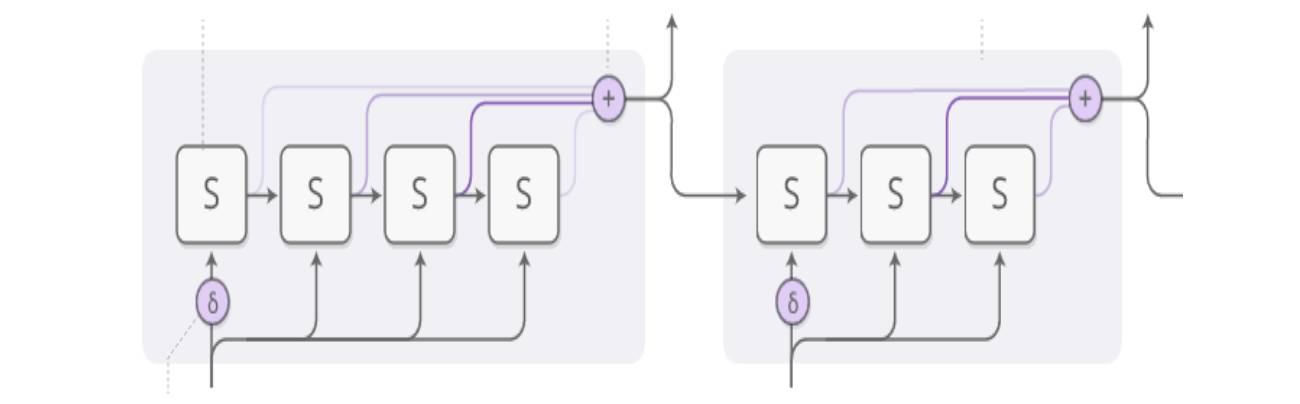
ACT-RNN Structure
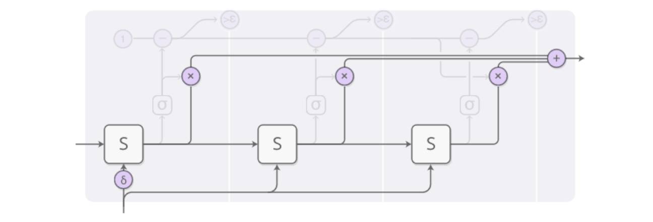
The above diagram illustrates a hidden layer structure with two-step propagation. It can be seen that the input at time T is split into 4 small steps for data input, marking the beginning of ACT.
Since the processing principle for each time step is consistent, we will now analyze each step’s specific process in detail:
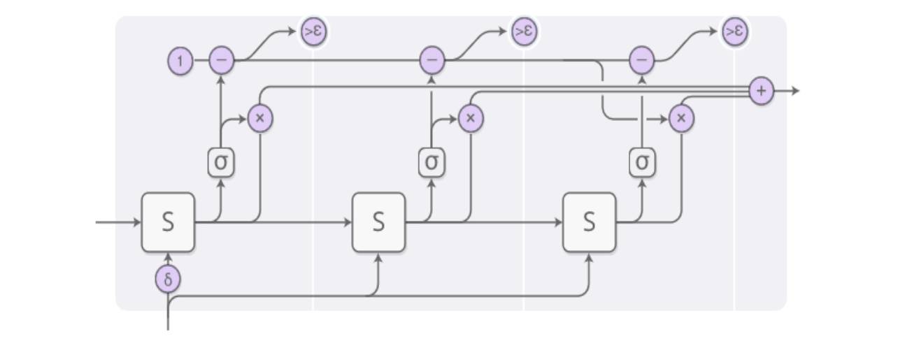
ACT-RNN Single-Step Structure
In an input at time T, as illustrated above, the final output after processing is composed of three outputs weighted together, all derived from the S-layer processing of the same input:
ACT-RNN Single-Step Structure Step 1
The weights for the three outputs are obtained through the sigmoid function shown below, referred to as the “halting neuron” in ACT.
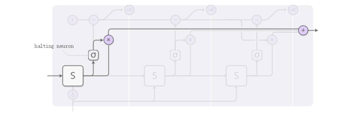
ACT-RNN Single-Step Structure Step 2
Since the main goal of ACT is to adaptively compute the number of calculations, as illustrated in the diagram, the cumulative probability provided by the halting neuron exceeds a threshold (epsilon), at which point the computation stops. The number of calculations before stopping is weighted, meaning that the number of outputs can vary.
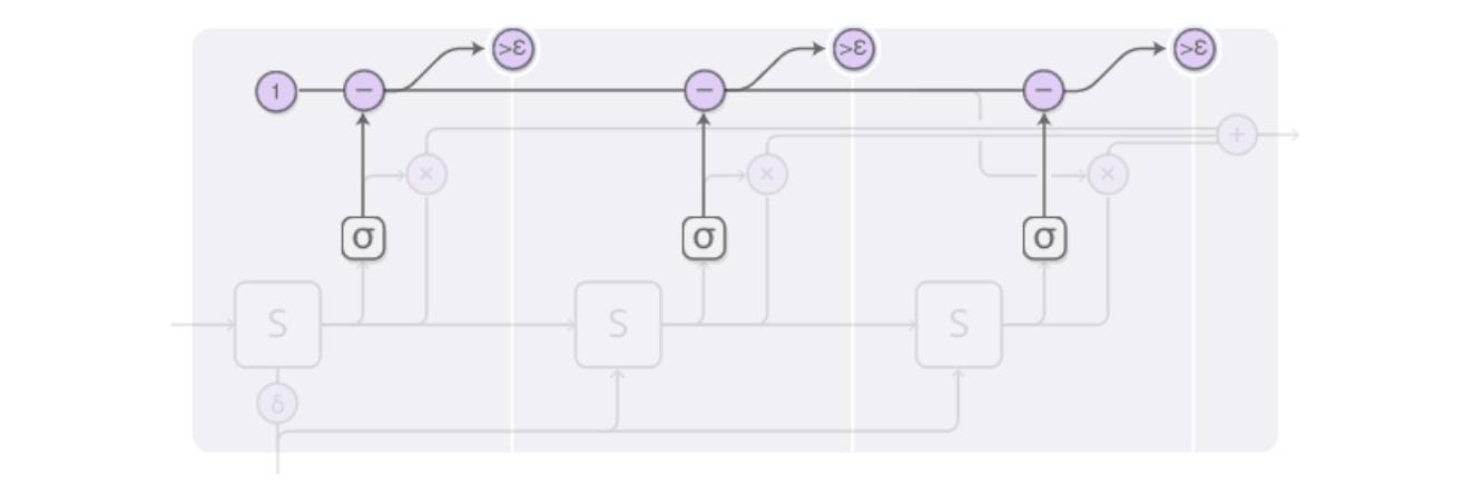 ACT-RNN Single-Step Structure Step 3
To summarize the entire process described above:
ACT-RNN Diagram
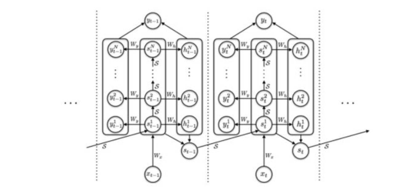
Each rectangle at each step indicates that the input Xt has been processed N times, with the final output st being a weighted sum of the st processed N times, thereby increasing the computational complexity of the network. The basic structure of traditional RNN is shown below:
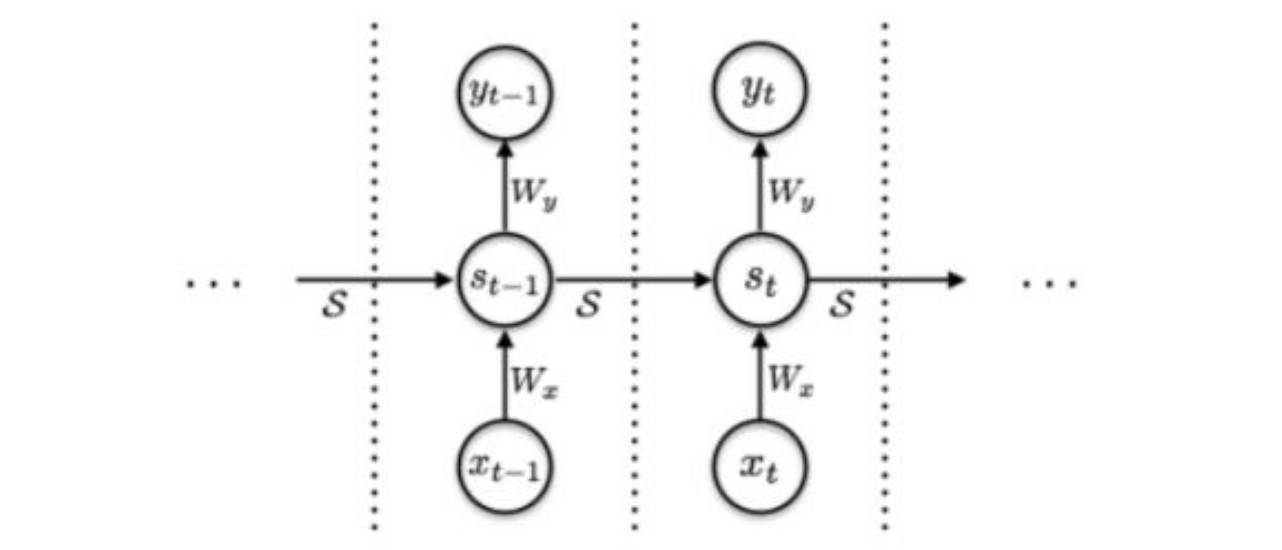
RNN Diagram
It can be seen that the traditional RNN structure does not have the rectangular structure shown in the previous image, but both maintain a consistent processing process over time.
Here, we will omit the strict mathematical definitions of the ACT model. Through the application of multi-factor models in the A-share market, we will directly observe the stock selection effect of the ACT RNN network and compare it with traditional RNN (LSTM) multi-factor stock selection models.
ACT-RNN Multi-Factor Stock Selection Model Parameters
Backtesting Period: May 1, 2007 – April 30, 2016, with over 180,000 monthly data training samples during this period (each stock at the end of each month represents one sample).
Strategy Period: May 1, 2016 – July 30, 2017
RNN Time Length (steps): 24 months, meaning each training sample includes factor data from the past 24 months, sequentially inputting from the first month into the neural network, and simultaneously looping the return value with the next month’s factor into the neural network, continuing until obtaining the prediction value for the 24th month.
Number of Factors: No merging of factors, excluding some factors with excessive correlation and belonging to the same category, which can reduce the likelihood of overfitting in model training. Ultimately, 48 small factors were selected, belonging to 10 common style factors.
Number of Classes: To verify the accuracy of predictions and exclude some noise from the samples, we divided the sample return types into three categories: Up (monthly return greater than 3%), Down (monthly return less than -3%), and Neutral. (After testing, the relative return label did not surpass the absolute return label during backtesting)
Batch Size: 1000, this parameter belongs to the system parameters of RNN neural networks and is used to calculate gradients in the BP algorithm. During each training, 1000 samples are randomly selected from the 180,000 training samples as training samples. Due to the structure of the ACT network, batch size has become a parameter that needs to be input into the ACT network.
Number of Hidden Layer Neurons: 400, 1 layer. This parameter also belongs to the system parameters of RNN neural networks, representing the number of “neurons” connecting input samples to hidden layer cells.
Basic RNN Cell:LSTM
Learning Rate: 0.0001, a system parameter of the RNN neural network, indicating the speed of gradient descent during model training. A rate that is too high may cause gradients to vanish, while a rate that is too low will slow down training.
Hesitation Threshold: 0.1, a parameter for ACT, meaning that when the cumulative value of the halting rate for each step of computation exceeds 0.9, the computation will stop.
Maximum Number of Calculations: 30, also a parameter for ACT, meaning that if the cumulative number of calculations reaches 30 for each period, the computation will stop. It works together with the hesitation threshold to control the number of calculations.
Stock Selection Effect
First, from the perspective of learning performance, compared to the LSTM network structure, the convergence speed of accuracy has increased. While ACT theoretically has the potential to enhance learning performance through increased network complexity, this is not guaranteed in practical applications. From this comparison, we can observe an increase in speed in multi-factor stock selection, with convergence improving from 7000 iterations for LSTM to below 5000 for ACT.
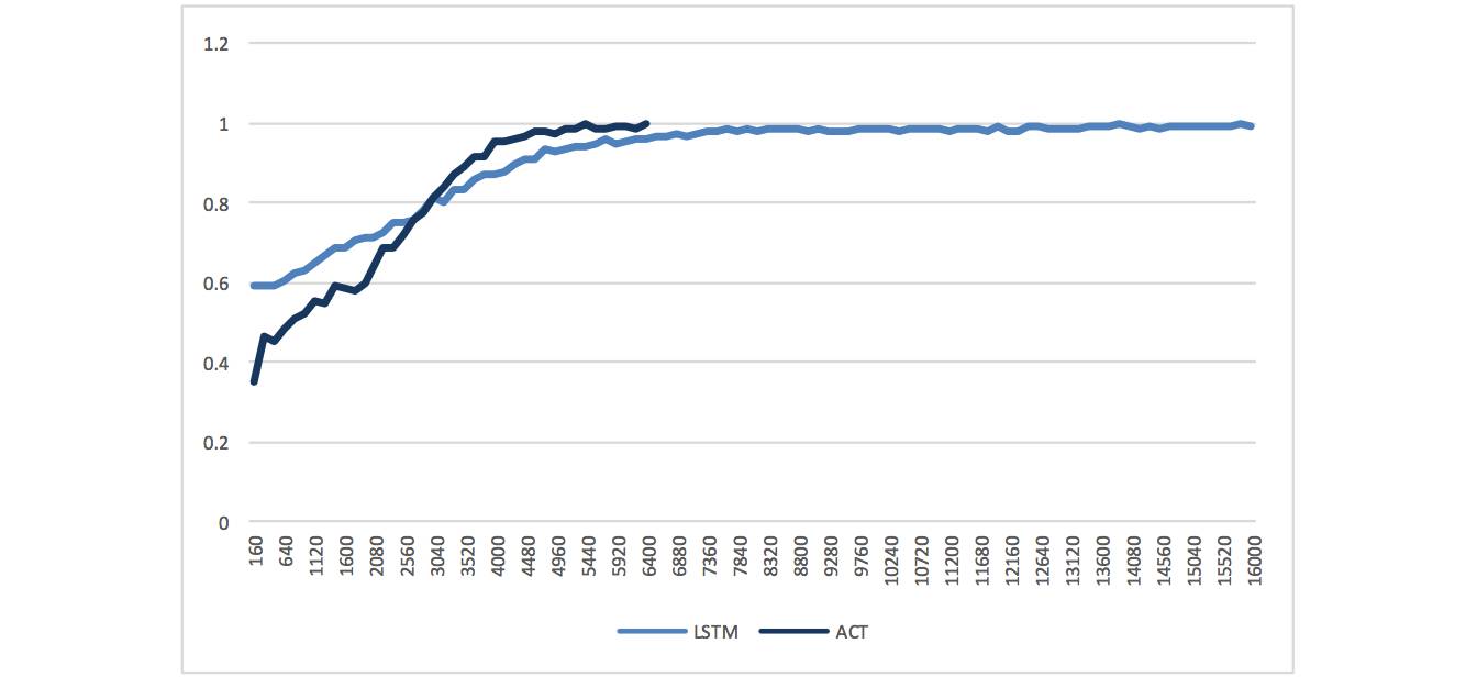
Training Accuracy Curve
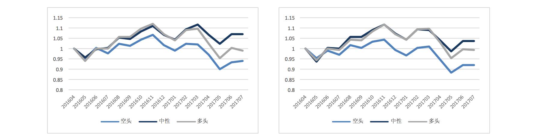
From the profit curves, we can observe more significant results compared to LSTM:
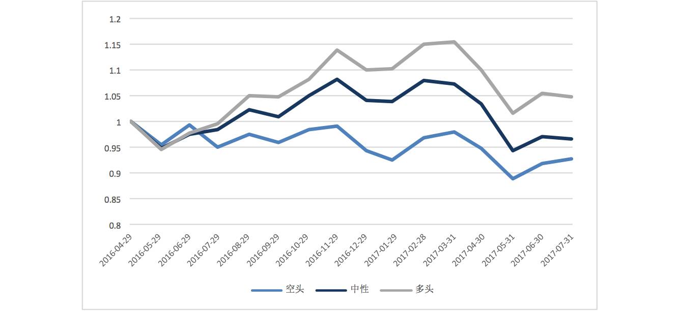
ACT Stock Selection
Ultimately, the profit curves for the bullish, bearish, and neutral categories can be significantly separated, and the absolute returns for the bullish combination are also significantly higher than those predicted by LSTM.
Stock Selection Feature Distribution
In machine learning algorithms, we evaluate the accuracy of a learning network by calculating the prediction results from all test samples. However, in stock selection, we are more concerned about the actual success rate of the algorithm’s predictions for bullish combinations.
Therefore, we choose to calculate the proportion of the top 100 stocks predicted by the algorithm to actually rise among the top 100 stocks, serving as a criterion for measuring the accuracy of the algorithm’s stock selection.
Bullish Combination TOP100 Accuracy
Unlike the cost function and accuracy calculated by the algorithm, we can see from the top 100 accuracy of the combination that the current RNN algorithm’s actual efficiency for bullish combinations is not outstanding, with the corresponding real accuracy averaging around 15%. This also explains the reason for the discrepancy between the algorithm’s high accuracy and the low value curve of the combination.
In addition to accuracy, the distribution of the proportion of stocks predicted to be bullish by the neural network for each period is shown in the following graph:
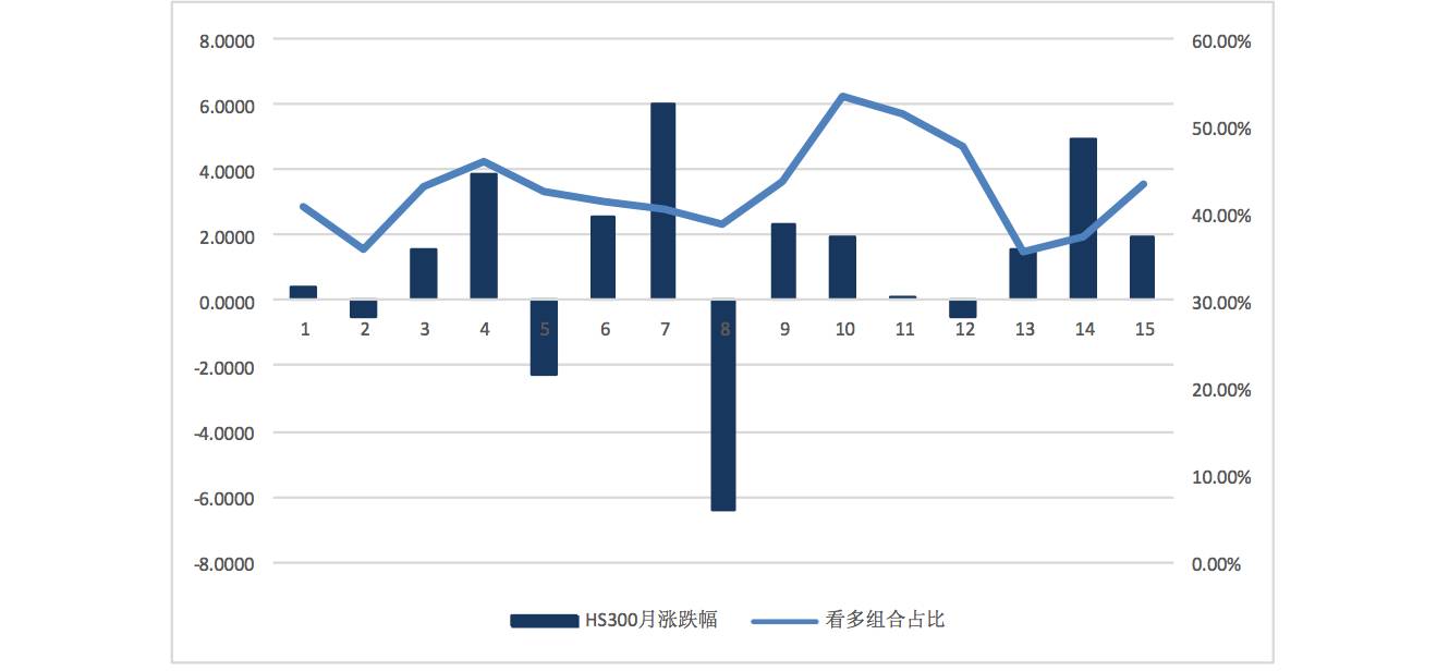
Bullish Combination Proportion
The average proportion of the combination is around 42%, while HS300 has a rise of over 30% in the past 15 months, with a proportion of about 33%. The RNN network tends to predict a higher proportion of bullish stocks. Meanwhile, comparing the actual rise and fall of the market index in the following months, we find that the proportion of bullish stocks predicted by the neural network correlates with the actual rise and fall of the market, with a 75% probability of this phenomenon occurring when the proportion of the combination increases.
Conclusion
The goal is to improve the structure of RNN and attempt to enhance the performance and results of the neural network.
Compared to the basic LSTM model, the main conclusion of this strategy relies on the enhanced structure ACT—Adaptive Computation Time. By increasing the number of repetitions for learning the same batch of data during each learning iteration, we enhance the complexity of the RNN network. From the results, it can be seen that the addition of ACT effectively improves the network’s ability to distinguish between bullish, bearish, and neutral combinations, and the actual return rate of the bullish combination has also improved compared to earlier reports.
Another approach is to improve the data structure at the input end. By attempting relative returns, optimizing the number of features, and shortening the time steps, we can achieve a certain degree of improvement, but the distinction of predicted combinations did not significantly improve.
However, it is still important to emphasize that for deep learning, increasing the complexity of the network structure is a major research direction, but the importance of data processing at the input end is even higher. The lack of good results from this strategy does not imply the failure of this direction; optimizing data processing is also worth continuing to explore and research.
Followers
From1to10000+
We are improving every day