The Transformer architecture has become a major component of the success of large language models (LLMs). To further improve LLMs, new architectures that may outperform the Transformer architecture are being developed. One such approach is Mamba, a state space model.
The paper “Mamba: Linear-Time Sequence Modeling with Selective State Spaces” introduces Mamba, which we have detailed in previous articles.
In this article, we will provide detailed comparisons by drawing architecture diagrams for RNNs, Transformers, and Mamba, allowing us to better understand the differences between them.
To illustrate why Mamba is such an interesting architecture, let’s first introduce the Transformer.
Transformer
The Transformer views any text input as a sequence of tokens.
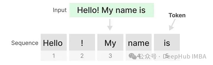
One major advantage of the Transformer is that it uses information from any token in the sequence to process the input data, regardless of how long the input is.
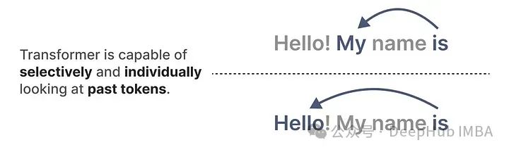
This is the role of the attention mechanism we see in the paper, but to obtain global information, the attention mechanism is very memory-intensive on long sequences, which we will discuss later.
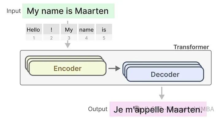
The Transformer consists of two structures: a set of encoder blocks for representing text and a set of decoder blocks for generating text. These structures can be used for various tasks, including translation.
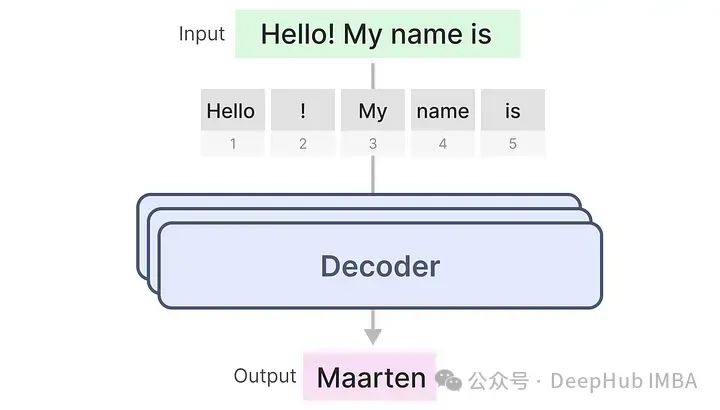
We can use this structure to create generative models that only use the decoder. For example, the Transformer-based GPT uses decoder blocks to complete some input text.
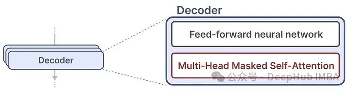
A single decoder block consists of two main parts: a self-attention module and a feedforward neural network.
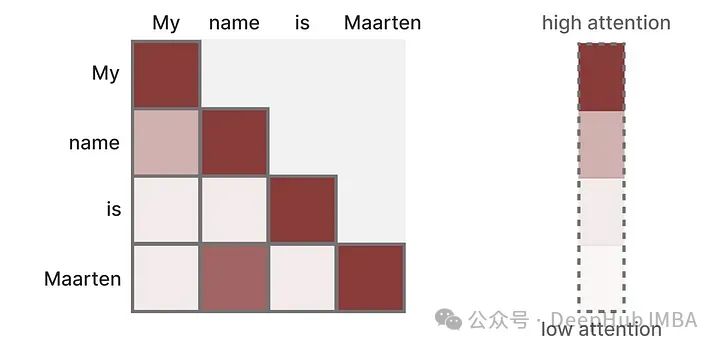
The attention mechanism creates a matrix that compares each token with every previous token. The weights in the matrix are determined by the relevance between token pairs.
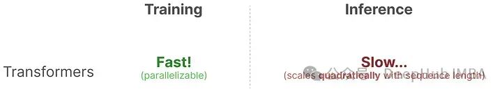
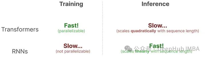
It supports parallelization, which can greatly speed up training!
However, when generating the next token, we need to recalculate the attention for the entire sequence, even if we have already generated some new tokens.
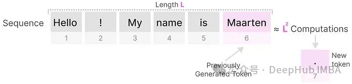
Generating tokens for a sequence of length L requires approximately L² computations; if the sequence length increases, the computation can become very large. Additionally, since all tokens’ attention needs to be calculated, memory usage can also be very high for long sequences. Thus, the need to recalculate the entire sequence is a major bottleneck of the Transformer architecture. Of course, there are many techniques to improve the efficiency of the attention mechanism, but we will not discuss them here, focusing only on the classic original paper.
RNN
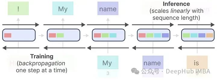
Next, we introduce the earlier sequence model, RNN. Recurrent Neural Networks (RNNs) are sequence-based networks. They take two inputs at each time step of the sequence: the input at time step t and the hidden state from the previous time step t-1, to generate the next hidden state and predict the output.
RNNs have a cyclical mechanism that allows them to pass information from the previous step to the next. We can “unfold” this visualization to make it clearer.
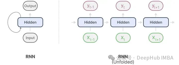
When generating outputs, RNNs only need to consider the previous hidden state and the current input. This avoids recalculating previous hidden states, which is something the Transformer does not have.
This process allows RNNs to perform quick inference because the time scales linearly with the sequence length! Furthermore, they can theoretically have an infinite context length, as each inference only takes one hidden state and the current input, resulting in very stable memory usage.
We will apply RNNs to the previously used input text.
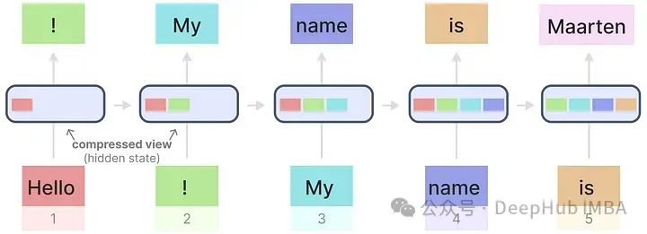
Each hidden state is an aggregation of all previous hidden states. However, a problem arises here: when generating the name “Maarten”, the last hidden state no longer contains information about the word “Hello” (or the earliest information gets overwritten by the latest). This leads to RNNs forgetting information over time because they only consider the previous state.
Moreover, the sequential nature of RNNs creates another problem. Training cannot be parallelized because it must be completed step by step in order.
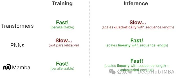
Compared to Transformers, RNNs have the opposite problem! Their inference speed is very fast, but the inability to parallelize leads to slow training.
People have been looking for a model that can train in parallel like Transformers, remember previous information, and still grow linearly in inference time with sequence length. Mamba is advertised as such.
Before introducing Mamba, let’s also introduce the state space model (SSM).
The State Space Model (SSM)
The state space model (SSM), like Transformers and RNNs, can process sequential information such as text and signals.
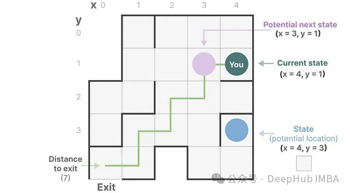
The state space is a concept that includes the minimum number of variables that can fully describe a system. It is a way to mathematically represent a problem by defining the possible states of the system.
For example, imagine we are navigating through a maze. The “state space” is a map of all possible positions (states). Each point represents a unique position in the maze, with specific details such as how far you are from the exit.
The “state space representation” is a simplified description of this map. It shows where you currently are (the current state) and where you can go next (the possible future).
Does this sound familiar? Isn’t this similar to the state in reinforcement learning? Personally, I think it can be understood this way. But how does it relate to sequences?
Because embeddings or vectors in language models are often used to describe the “state” of the input sequence. For instance, your position vector (state vector) might look like this:

In neural networks, “state” usually refers to its hidden state, which is one of the most important aspects of generating new tokens in the context of large language models.
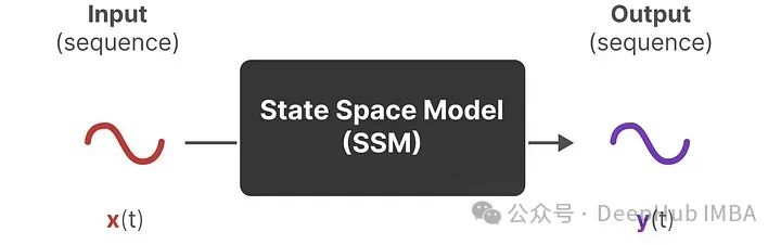
State space models (SSMs) are used to describe these state representations and predict the next state based on certain inputs.
At time t, a state space model (SSM):
-
maps the input sequence x(t) (for example, moving left and down in the maze) to a latent state representation h(t) (for example, the distance to the exit and x/y coordinates),
-
and derives the predicted output sequence y(t) (for example, moving left again to reach the exit faster).
Here, it differs from reinforcement learning, which uses discrete sequences (like moving left once) by taking continuous sequences as input and predicting output sequences.
The SSM assumes that a dynamic system, such as a moving object in three-dimensional space, can be predicted from the state at time t using two equations.

By solving these equations, assumptions can reveal statistical principles for predicting the system’s state based on observed data (input sequences and previous states).
The goal is to find this state representation h(t) so that we can map from an input sequence to an output sequence.
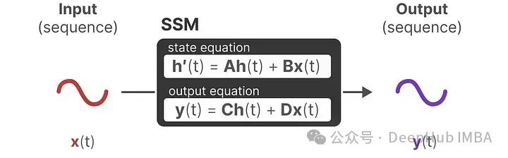
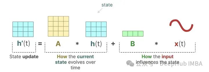
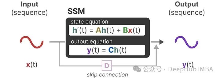
These two equations are the core of the state space model. The state equation describes how input affects the state change (through matrix B) and how the state is influenced (through matrix A).
h(t) represents the latent state representation at any time t, while x(t) represents some input.
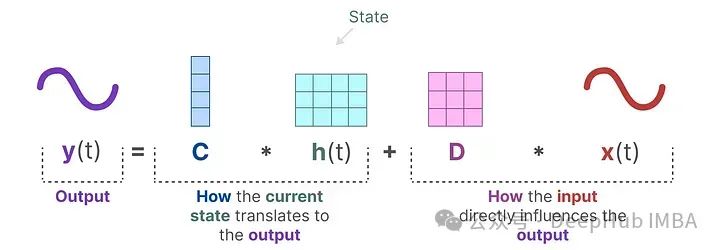
The output equation describes how the state is transformed into output (through matrix C) and how the input affects the output (through matrix D).
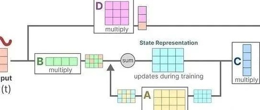
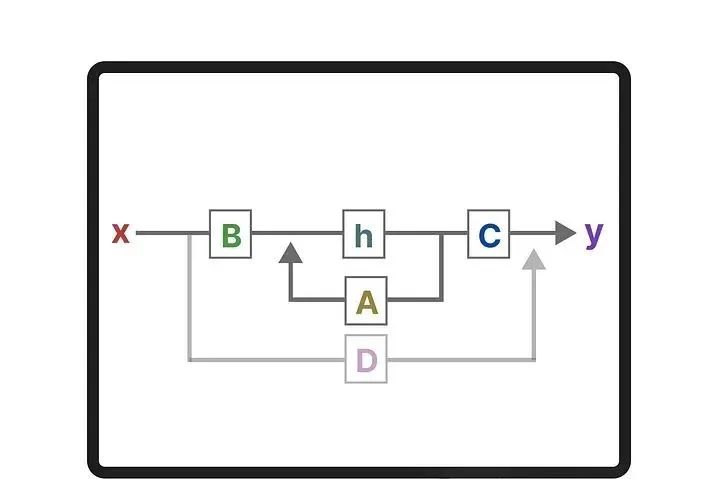
The matrices A, B, C, and D are often referred to as parameters because they are learnable. Visualizing these two equations, we can obtain the following architecture:

Next, let’s look at how these matrices influence the learning process.
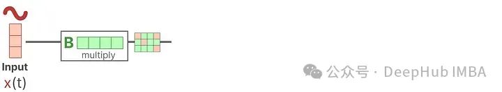
Suppose we have an input signal x(t). This signal is first multiplied by matrix B, which describes how the input affects the system.
The updated state (h) contains the core “knowledge” of the environment in latent space. We multiply the state by matrix A, which describes how all internal states are connected, as they represent the system’s latent representation.
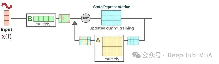
Here we can see that matrix A is applied before creating the state representation and updated after the state representation is updated.
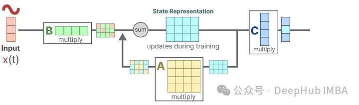
Then, we use matrix C to describe how to convert the state into output.
Finally, we utilize matrix D to provide a direct signal from input to output. This is often referred to as a skip (residual) connection.
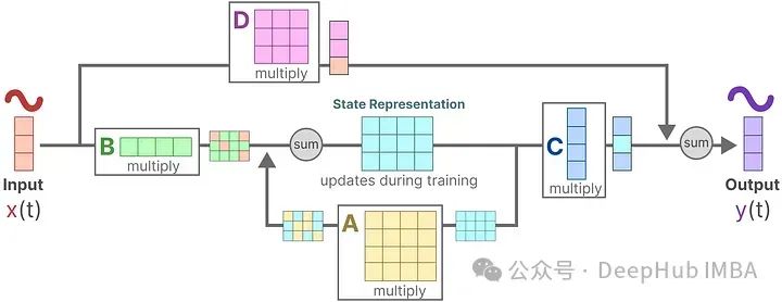
Since matrix D is similar to a skip connection, SSMs are often viewed as the parts that do not perform skip connections.
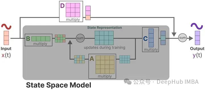
Returning to our simplified view, we can now focus on matrices A, B, and C, which are the core of SSM.

Updating the original equations and adding some color to indicate the purpose of each matrix.
These two equations predict the state of the system based on observed data. Since the expected input is continuous, SSM is a continuous-time representation.
However, since text is discrete input, we also need to discretize the model. This is where the *Zero-order hold* technique comes into play.
Every time we receive a discrete signal, we ensure its value remains unchanged until we receive a new discrete signal to change it. This process creates a continuous signal that SSM can use:
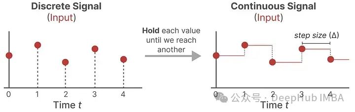
The duration for which we hold that value is represented by a new learnable parameter called the step size ∆. This results in a continuous signal that can sample values based solely on the input time step.
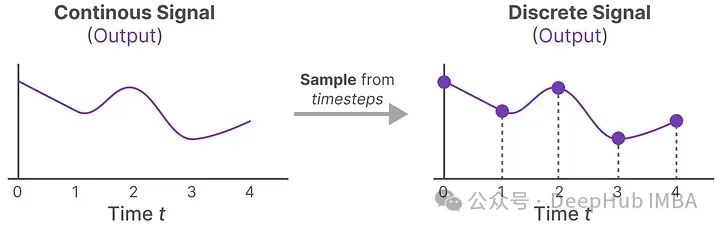
These sampled values are our discrete outputs! Mathematically, we can apply Zero-order hold as follows:
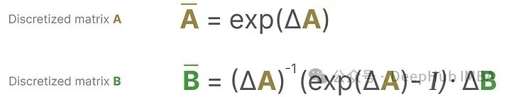
Since our SSM processes discrete signals, this is not a function to function mapping, x(t)→y(t), but rather a sequence to sequence mapping, xₖ→yₖ, which we express mathematically as:
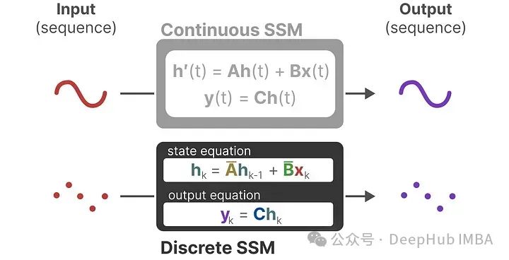
Now, matrices A and B represent the discrete parameters of the model, replacing t with k to indicate discrete time steps.
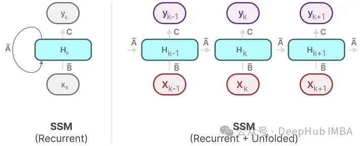
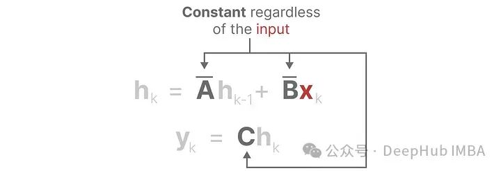
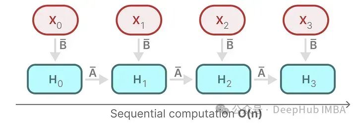
Discretizing the SSM allows for processing information at specific time steps. Just like we saw earlier with Recurrent Neural Networks (RNNs), a recurrent approach is also very useful here to rephrase the problem in terms of time steps:
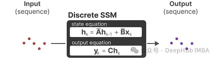
At each time step, we calculate how the current input (Bxₖ) affects the previous state (Ahₖ₁), and then calculate the predicted output (Chₖ).
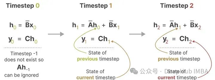
Does this representation look familiar? It actually processes similarly to RNNs.
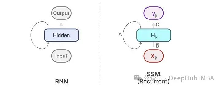
It can also be unfolded like this:
This technique is similar to RNNs, allowing for quick inference and slow training.
Another representation of SSM is the convolutional representation. We apply filters (kernels) to obtain aggregated features:
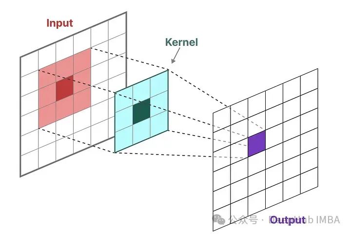
Since we are dealing with text rather than images, we only need a one-dimensional perspective:
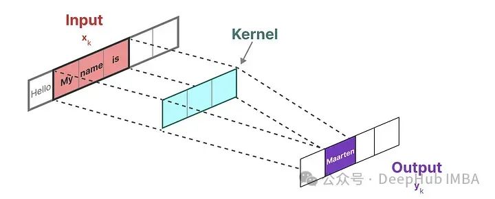
The kernel we use to represent this “filter” is derived from the SSM formula:
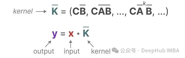
We can use the SSM kernel to traverse each group of tokens and compute the output:
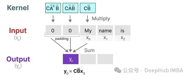
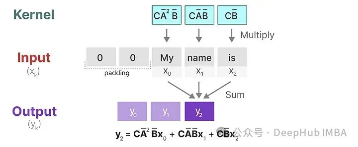
The above illustration also shows how padding can affect output, so we generally pad at the end rather than at the front. The second kernel is moved once to perform the next computation:

In the final step, we can see the complete effect of the kernel:
A major benefit of convolution is that it allows for parallel training. However, due to the fixed kernel size, their inference is not as fast as RNNs and has limitations on sequence length.
The above three SMMs each have their own advantages and disadvantages.
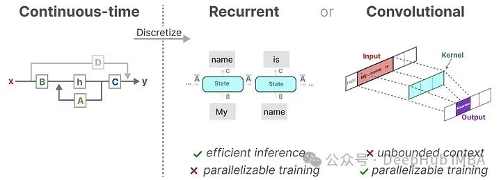
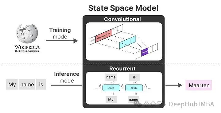
Here, a simple technique can be used to choose representations based on the task. During training, we use a convolutional representation that can be parallelized, and during inference, we use an efficient recurrent representation:
It sounds a bit fantastical, but someone has actually implemented it. This model is called the Linear State-Space Layer (LSSL).
https://proceedings.neurips.cc/paper_files/paper/2021/hash/05546b0e38ab9175cd905eebcc6ebb76-Abstract.html
It combines the theory of linear dynamic systems with the concepts of neural networks, effectively capturing temporal information and dynamic features in the data. LSSL is based on linear dynamic system theory, which can be represented using state space models. In this model, the system’s behavior is determined by the evolution of state variables and the influence of external control signals. The state variables are the internal representations of the system, capturing its dynamic characteristics.
These representations have an important property, namely linear time invariance (LTI). LTI means that the SSM parameters A, B, and C are fixed for all time steps. This means that for each token generated by the SSM, matrices A, B, and C are the same.
In other words, regardless of the sequence given to the SSM, the values of A, B, and C remain unchanged. This results in a static representation that does not consider content. However, static representations are meaningless, right? So Mamba addresses this issue. However, before introducing Mamba, we need to emphasize one more knowledge point: matrix A.
Because the most important aspect of the SSM formula is matrix A. As we saw earlier in the recurrent representation, it captures information about the previous state to build a new state. If matrix A forgets information from very early on, just like RNNs do, then SMM will have no meaning, right?

Matrix A generates hidden states:

How can we create matrix A to retain a large context size?
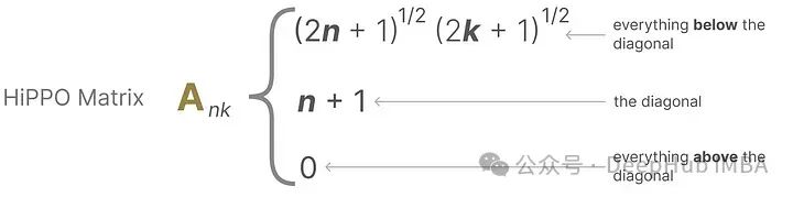
The HiPPO model combines the concept of recursive memory with optimal polynomial projections, which can significantly improve the performance of recursive memory, especially when dealing with long sequences and long-term dependencies.
https://proceedings.neurips.cc/paper/2020/hash/102f0bb6efb3a6128a3c750dd16729be-Abstract.html
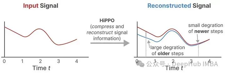
Using matrix A to construct a state representation that can effectively capture recent tokens while decaying older tokens can be expressed as:
We will not go into the specific details here; those interested can refer to the original paper.
Thus, we have basically solved all the problems: 1. State space models; 2. Handling remote dependencies; 3. Discretization and parallel computation.
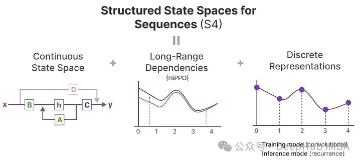
If you want to learn more about how to compute the HiPPO matrix and build the S4 model yourself, I recommend reading the annotated S4.
https://srush.github.io/annotated-s4/
Mamba
After introducing all the necessary foundations, we finally arrive at our main focus.
Mamba has two main contributions:
1. A selective scanning algorithm that allows the model to filter relevant and irrelevant information.
2. A hardware-aware algorithm that effectively stores (intermediate) results through parallel scanning, kernel fusion, and recomputation.
Before discussing these two main contributions, let’s first look at why they are necessary.
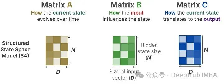
The state space model, S4 (Structured State Space Model), performs poorly on certain tasks in language modeling and generation.
For instance, in the selective copying task, the goal of SSM is to sequentially copy parts of the input and output:
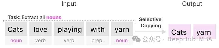
(Recurrent/Convolutional) SSM performs poorly on this task because it is linear time-invariant. For each token generated by SSM, matrices A, B, and C are the same.
Because it treats each token equally as a result of fixed matrices A, B, and C, SSM cannot perform content-aware inference.
The second task where SSM performs poorly is reproducing patterns found in the input:
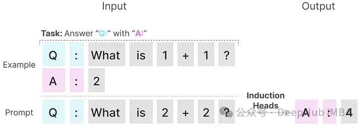
Our prompts teach the model to provide an “A:” response after each “Q:”. However, because SSM is time-invariant, it cannot selectively retrieve previous tokens from its history.
For example, matrix B remains completely the same regardless of the input x:
Similarly, matrices A and C also remain unchanged regardless of the input, which is what we referred to as static.
In contrast, Transformers can dynamically change attention based on the input sequence. They can selectively “look at” or “attend to” different parts of the sequence, and the addition of position encoding makes Transformers very straightforward for such tasks.
The poor performance of SSM on these tasks highlights the potential issues with stationary SSMs, where the static characteristics of matrices A, B, and C lead to content-aware problems.
Selective Information Retention
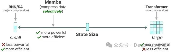
The recurrent representation of SSM creates a very efficient small state because it compresses the entire historical information. Thus, its functionality is much weaker than that of a Transformer model that does not compress history (the attention matrix).
The goal of Mamba is to achieve a “small” state as powerful as that of Transformers.
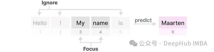
By selectively compressing data into the state, when inputting a sentence, there are often some pieces of information, such as stop words, that carry little significance.
Let’s first look at the input and output dimensions during the training period of SSM:

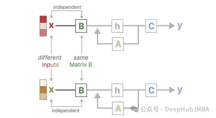
In the Structured State Space Model (S4), matrices A, B, and C are independent of the input because their dimensions N and D are static and do not change.
In contrast, Mamba makes matrices B and C, and even the step size ∆, dependent on the input by combining the sequence length and batch size:
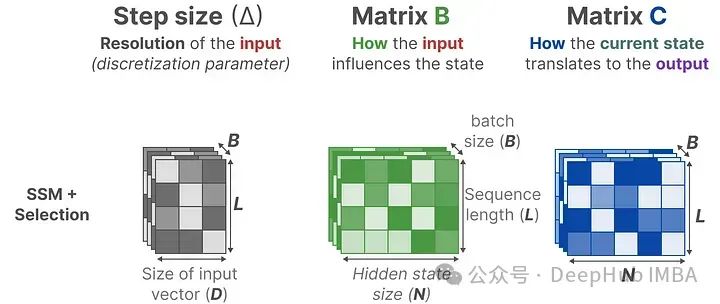
This means that for each input token, there are different matrices B and C, which solves the content-aware problem! Here, matrix A remains unchanged because we want the state itself to remain static, but the way it is influenced (via B and C) is dynamic.
In other words, they together selectively choose what to retain in the hidden state and what to ignore, all determined by the input.
A smaller step size ∆ leads to ignoring specific words, relying more on previous context, while a larger step size ∆ focuses more on the input words rather than the context:
Scanning Operation
Now that these matrices are dynamic, they cannot be computed using convolutional representation and can only be processed using recurrence, which makes parallelization impossible.
To achieve parallelization, let’s first look at the output of the recurrence:
Each state is the sum of the previous state (multiplied by A) and the current input (multiplied by B). This is called the scanning operation, which can easily be computed through a for loop. However, parallelization seems impossible, as each state can only be computed when we have the previous state.
However, Mamba uses parallel scanning, assuming that the order of operations does not matter due to associativity. This allows for partial sequences to be computed and iteratively combined:
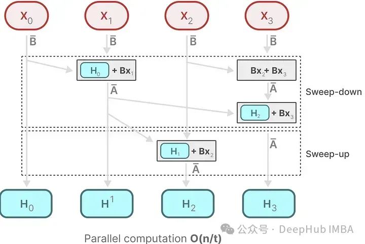
Another advantage is that since the order does not matter, we can also omit the position encoding of the Transformer.
Hardware-Aware Algorithms
A recent drawback of GPUs is their limited transfer (IO) speed between small but efficient SRAM and large but slightly less efficient DRAM. Frequent copying of information between SRAM and DRAM has become a bottleneck.
The specific allocation of Mamba’s DRAM and SRAM is as follows:
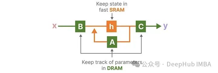
Intermediate states are not saved, but they are necessary for computing gradients during backpropagation. The authors recompute the intermediate states during the backpropagation process. Although this may seem inefficient, it is much cheaper than reading all these intermediate states from the relatively slow DRAM.
We will not elaborate on this part, as I have not researched it much.
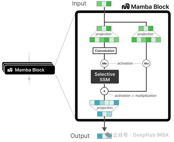
Mamba Blocks
The selective SSM can be treated as a block, similar to the attention module in Transformers. We can stack multiple blocks and use their outputs as inputs to the next Mamba block:
The final end-to-end (input to output) example includes normalization layers and a softmax output layer for selecting output tokens.
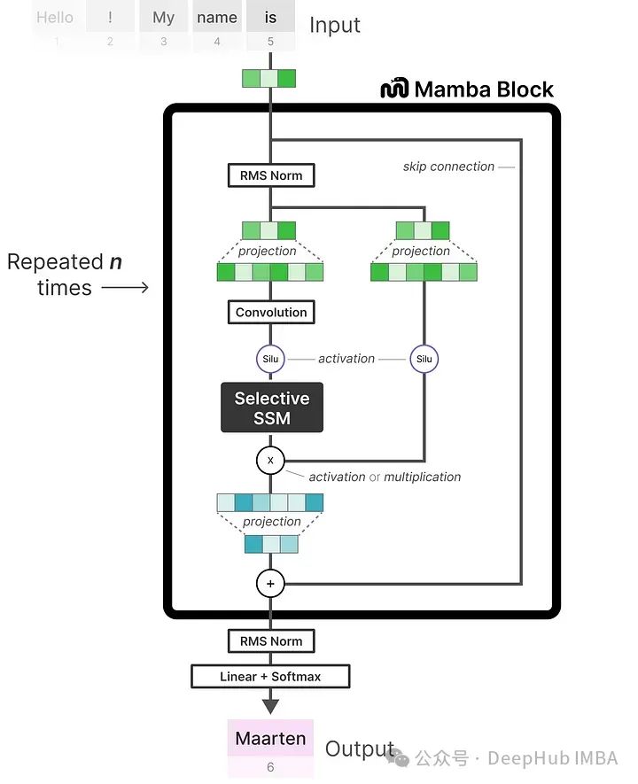
This results in a model with fast inference and training, capable of handling “infinite” length contexts.
Conclusion
After reading this article, I hope you have gained a certain understanding of Mamba and state space models. Finally, we conclude with the author’s discovery:
The author found that the model performs comparably to Transformer models of the same size and sometimes even outperforms them!
Author: Maarten Grootendorst
Editor: DeepHub IMBA