Skip to content
Selected from Reddit
Translated by Machine Heart
Contributors: Wang Zhi Jia, Mo Wang
A study from Stanford University found a correspondence between waves in physics and computations in RNNs.
Paper link:https://advances.sciencemag.org/content/5/12/eaay6946
GitHub link:https://github.com/fancompute/wavetorch
Recently, there has been a lot of exciting interaction between machine learning and some fields of physics and numerical sciences. This has allowed machine learning frameworks to be applied to the optimization problems of physical models, while many exciting new models in the machine learning field have emerged with the help of physical concepts (e.g., neural ODEs and Hamiltonian neural networks).
The research focus of the author’s group is that physics itself can serve as a computational engine. In other words, the authors are interested in physical systems that can act as hardware accelerators (or specialized processors designed for fast and efficient machine learning computations).
In their recently published paper in Science Advances, they demonstrated that the physical properties of waves can be directly mapped to the temporal changes in recurrent neural networks (RNNs). Using this connection, the authors developed a numerical model with PyTorch that shows we can train an acoustic/optical system to accurately recognize vowels from recordings of human speakers. Essentially, the authors introduced vowel waveforms into a physical model and allowed the optimizer to add and remove materials at 1000 points within the domain, which can effectively act as the weights of the model.
Since this machine learning model corresponds to a physical system, it also means that researchers can “print” the trained material distribution onto real physical devices. The result is similar to an ASIC (Application Specific Integrated Circuit) but is specific to certain RNN computations. This is very exciting because these results suggest that complex recurrent machine learning computations can be performed without consuming excess energy (other than the energy carried by the pulse itself).
Below is an introduction to the core ideas of this research.
Connection Between Waves and RNNs
This section will introduce the connection between the operations of RNNs and waves.
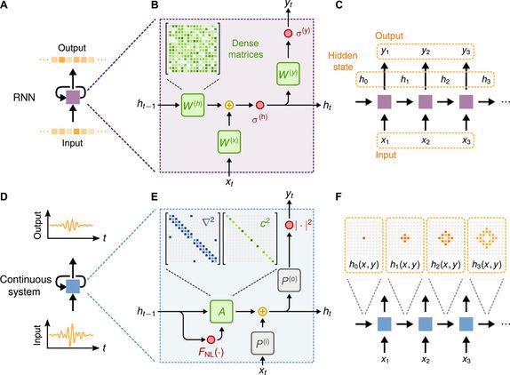
RNNs execute the same operation on each part of the input sequence step by step, converting the input sequence into an output sequence (Figure 1A). The information from previous steps is encoded and stored in the hidden state of the RNN, which is updated at each step. It is these hidden states that allow the RNN to remember past information while learning the temporal structure and long-distance dependencies in the data. At a given time step t, the RNN processes the current input vector x_t from the input sequence and the hidden state vector h_t-1 from the previous step simultaneously, producing the output vector y_t and updating the current hidden state h_t.
Figure 1:Conceptual comparison between standard RNNs and wave-based physical systems.
Training a Physical System to Recognize Vowels
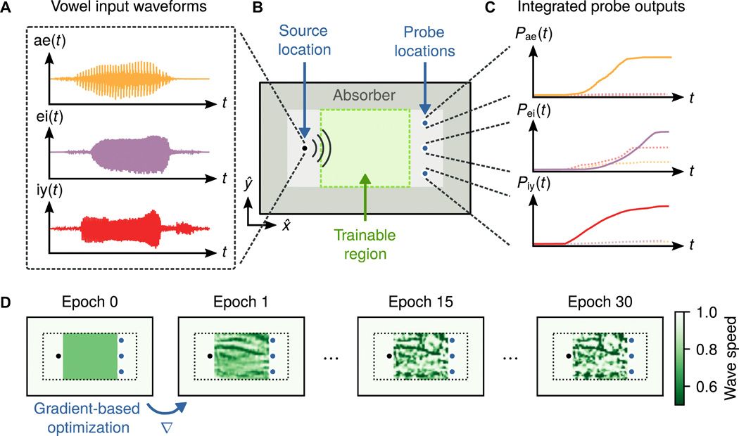
This section will explain how to use wave equations to train a vowel classifier, primarily through constructing a non-uniform material distribution. To accomplish this task, the dataset used in the study includes 930 raw recordings of 10 vowels from 45 male and 48 female speakers. During the model training process, the study selected 279 recordings related to 3 vowels (ae, ei, iy) as the training set (Figure 2A).
Figure 2:Setup and training process for vowel recognition.
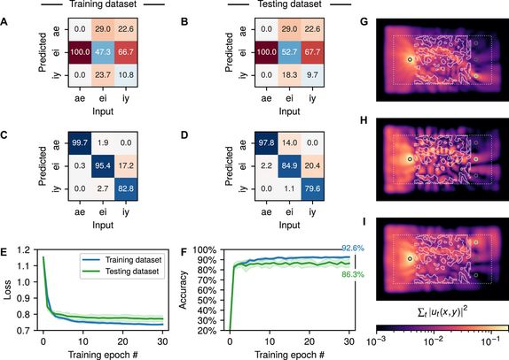
The confusion matrix obtained by averaging the results of 5-fold cross-validation training on both the training set and test set is shown in Figure 3 (A, B). The values on the diagonal of the confusion matrix define the proportion of correctly predicted vowels, while the values off the diagonal represent the proportion of failures to predict correctly. The results indicate that the initial structure is unable to complete the recognition task.
Figures C and D in Figure 3 show the final confusion matrices on the optimized training set and test set. These results are also averages from 5-fold cross-validation runs. The trained confusion matrix is diagonally dominant, meaning that this structure can now perform the vowel recognition task.
Figure 3:Training results for the vowel recognition task.
Figures E and F in Figure 3 display the cross-entropy loss and prediction accuracy, with the x-axis representing the number of training epochs on the training set and test set. The solid lines in the figure represent averages, while the shaded areas indicate the standard deviation of the cross-validation training runs. From this, we see that the first epoch resulted in the largest drop in loss and the greatest improvement in accuracy. From Figure 3F, we can see that the average accuracy of this system on the training set is 92.6 ±1.1%, while the average accuracy on the test set is 86.3 ± 4.3%.
From Figures C and D in Figure 3, it can be observed that the system performs nearly perfectly in recognizing the vowel ae and can differentiate iy and ei well (though with slightly lower accuracy), a feature that is particularly evident on unseen samples in the test set. Figures G to I in Figure 3 show the integrated field intensity ∑_t u_t^2 when representative samples of each vowel class are injected into the training structure.
The study visually demonstrated that the optimization process to produce the target structure directs most of the signals to the correct locations. This task used the traditional RNN as a performance benchmark, and its classification accuracy is comparable to that of the wave equation, but it requires a large number of free parameters. Additionally, we observed that the classification accuracy obtained from training the linear wave equation is also highly competitive, with more details on performance available in the original paper.
The wave-based RNN proposed in this study has many advantages that allow it to excel in handling temporal encoded information. Unlike traditional RNNs, the wave equation achieves nearest-neighbor coupling between hidden state elements during the update process from one time step to another through the Laplacian operator (the sparse matrix in Figure 1E). The nearest-neighbor coupling primarily benefits from the fact that wave equations are hyperbolic partial differential equations where information propagates at finite speeds. Therefore, the size of the hidden state and storage capacity simulating RNNs directly depends on the size of the propagating medium. Furthermore, unlike traditional RNNs, the wave equation adheres to energy conservation constraints, preventing the norms of hidden states and output signals from growing indefinitely. In contrast, the unconstrained dense matrices defining the update relationships of standard RNNs can lead to vanishing and exploding gradients, which are major challenges in the training process of traditional RNNs.
This study proves that wave equations are conceptually equivalent to RNNs. This conceptual connection provides ideas for a new class of analog hardware platforms, where the evolution of time sequences plays an important role in both physics and datasets. When we focus on the most general wave examples described by scalar wave equations, our results can be easily extended to other physical concepts similar to waves. This method of utilizing physics to perform computations may facilitate the development of new platforms for analog machine learning devices, which are expected to execute computations more naturally and efficiently than their digital counterparts. The generality of this method further suggests that many physical systems may be strong candidates for performing RNN-like computations on dynamic signals (such as those in optics, acoustics, or seismology).
Reference Links:https://www.reddit.com/r/MachineLearning/comments/ej3bgf/r_acoustic_optical_and_other_types_of_waves_are/
This article is compiled by Machine Heart, please contact this public account for authorization to reprint
Submissions or inquiries for reports: content@jiqizhixin.com