1.Origin
Transformers are an important deep learning architecture that originated in the fields of computer science and artificial intelligence. They have achieved remarkable success in natural language processing and other sequential data tasks. The history and evolution of this architecture are worth exploring.
The story of Transformers began in 2017, when Vaswani et al. first proposed the concept in their paper “Attention Is All You Need.” This paper introduced a novel attention mechanism called Self-Attention to replace traditional recurrent and convolutional structures. This innovative idea led to a revolution in deep learning, particularly in the fields of sequence modeling and natural language processing.
2. Transformer Principles
2.1 Overall Structure of Transformer
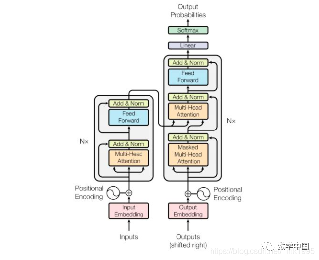
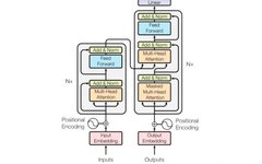
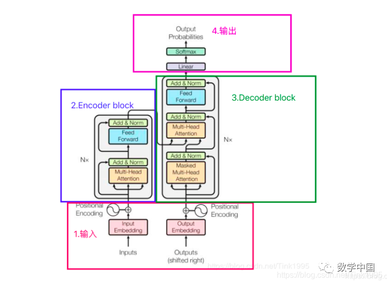
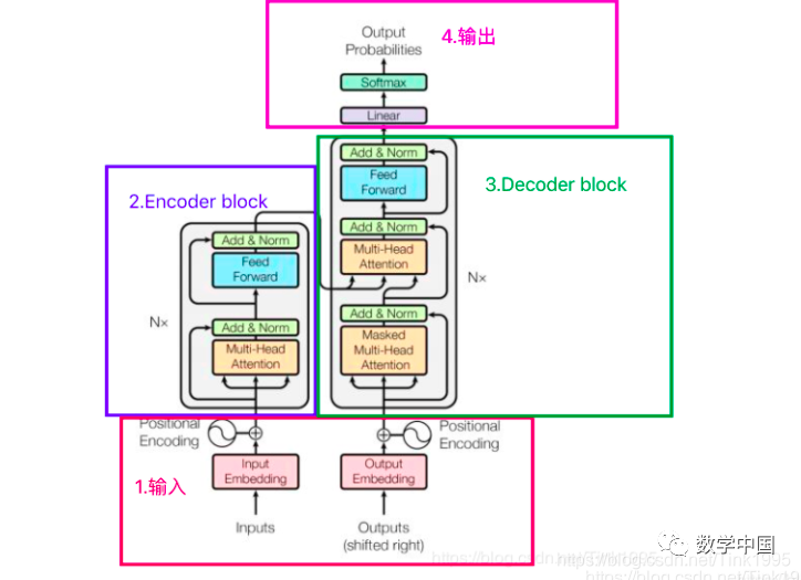
The above image shows the complete structure of the Transformer. Are you confused? What is all this? Don’t leave yet! Let’s tackle the Transformer step by step.
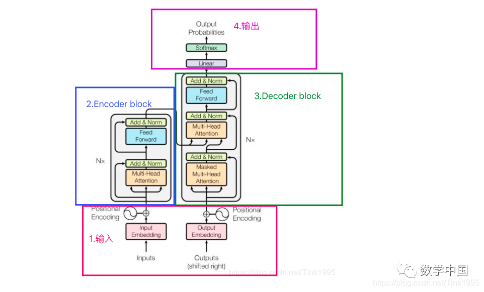
The structure diagram of the Transformer can be broken down into four main parts, with the most important being parts 2 and 3, the Encoder-Decoder sections. Yes, the Transformer is a model based on the Encoder-Decoder framework.
Next, I will introduce the network structure of the Transformer in the order of 1, 2, 3, and 4, which will help clarify the structural principles and facilitate understanding of the workflow of the Transformer model.
2.2 Inputs of the Transformer
The input to the Transformer is a sequence of data. For example, translating “Tom chase Jerry” into Chinese as “汤姆追逐杰瑞”:
The inputs to the Encoder are the word vectors obtained from tokenizing “Tom chase Jerry.” These can be in any form of word vectors, such as word2vec, GloVe, or one-hot encoding.
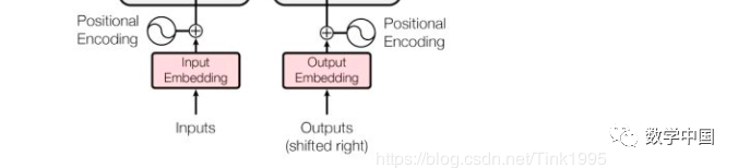
Assuming that each word vector in the above image is a 512-dimensional vector.
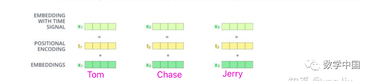
We note that after embedding the input vectors, we need to add positional encoding to each word vector. Why is positional encoding necessary?
First, we know that in a sentence, if the same word appears in different positions, the meaning can change dramatically. For example: “I owe him 100W” and “He owes me 100W” have completely different meanings. Thus, obtaining the positional information of words in a sentence is crucial. However, the Transformer is entirely based on self-attention, which cannot capture the positional information of words. Even if the positions of words in a sentence are shuffled, each word can still compute attention values with others, effectively acting as a powerful bag-of-words model without any impact on the results (this will be explained in more detail when discussing the Encoder). Therefore, we need to add positional encoding to each word vector during input.
Now the question arises: How do we obtain this positional encoding?
1. Positional encoding can be learned through data training, similar to how word vectors are learned. Google’s BERT uses learned positional encoding.
2. In the paper “Attention Is All You Need,” the Transformer uses sinusoidal positional encoding. Positional encoding is generated using sine and cosine functions of different frequencies, which are then added to the corresponding word vectors. The dimensions of the positional vectors must match those of the word vectors. The process is shown in the above image, and the calculation formula for PE (positional encoding) is as follows:
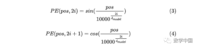
To explain the formula above:
pos represents the absolute position of a word in the sentence, where pos=0,1,2… For example, Jerry in “Tom chase Jerry” is pos=2; dmodel represents the dimensionality of the word vectors, in this case dmodel=512; 2i and 2i+1 represent odd and even indices, where i indicates the dimension of the word vector, for example, here dmodel=512, thus i=0,1,2…255.
As for how this formula was derived, it is not crucial because it is likely that the authors created it based on experience, and the formula is not unique. Later, Google’s BERT did not use this method for positional encoding but instead learned PE through training, indicating that there are still optimization opportunities with this method.
Here, I won’t go into detail. For those who want to delve deeper, you can refer to these answers on Zhihu: How to understand the positional encoding in the Transformer paper, and what is its relationship with trigonometric functions?
Why do we add positional encoding to the word vectors instead of concatenating them?
Both concatenation and addition are possible; however, since the dimensionality of the word vectors is already large at 512 dimensions, concatenating an additional 512-dimensional positional vector would result in a 1024-dimensional vector, which would slow down training and affect efficiency. The effects of both methods are similar, so it makes sense to choose the simpler addition approach.
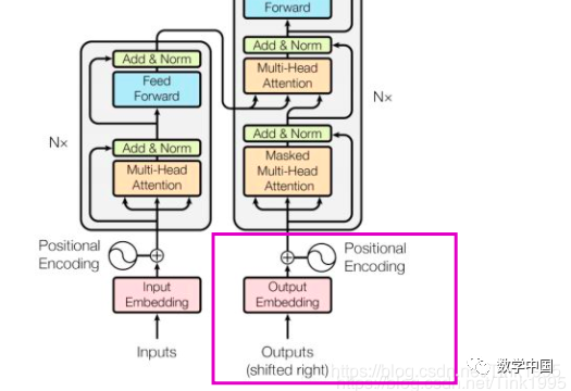
The input to the Transformer’s Decoder is processed in the same way as the Encoder’s output. One accepts source data, while the other accepts target data. In the above example, the Encoder receives the English “Tom chase Jerry,” while the Decoder receives the Chinese “汤姆追逐杰瑞.” During supervised training, the Decoder will also accept Outputs Embedding, but it will not receive this during prediction.
Thus, we have completed the explanation of the input section of the Transformer. Next, we will enter the key components: the Encoder and Decoder.
2.2 Encoder of the Transformer
Looking at the Encoder block in the second part of the above image. The Encoder block consists of six encoders stacked together, Nx=6. The gray box in part 2 of the image shows the internal structure of an encoder. From the diagram, we can see that an encoder is composed of Multi-Head Attention and a fully connected neural network called the Feed Forward Network.
Multi-Head Attention:
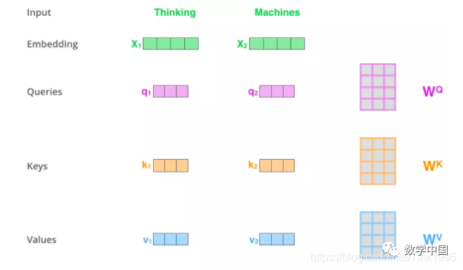
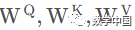
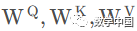
First, let’s review self-attention. Suppose the input sequence is “Thinking Machines,” where x1 and x2 correspond to “Thinking” and “Machines” after adding positional encoding to the word vectors. The word vectors are transformed into Query, Keys, and Values vectors required for calculating attention values through three weight matrices.
Since in practical usage, each sample, i.e., each sequence of data, is input in matrix form, we can see that the X matrix consists of the word vectors for “Thinking” and “Machines,” which are then transformed to obtain Q, K, and V. Assuming the word vectors are 512-dimensional, the dimension of the X matrix is (2,512).
Q, K, and V will all be (2,64)-dimensional.
After obtaining Q, K, and V, the next step is to calculate the attention values.
Step 1: Calculate the relevance scores between each word in the input sequence. As mentioned previously, the dot product method can be used to calculate the relevance scores, which involves calculating the dot product of each vector in Q with every vector in K. Specifically, in matrix form:
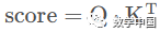
Here, score is a (2,2) matrix.
Step 2: Normalize the relevance scores between each word in the input sequence. Normalization is primarily aimed at stabilizing gradients during training.
Here, dk represents the dimension of K, which is assumed to be 64 in the above example.
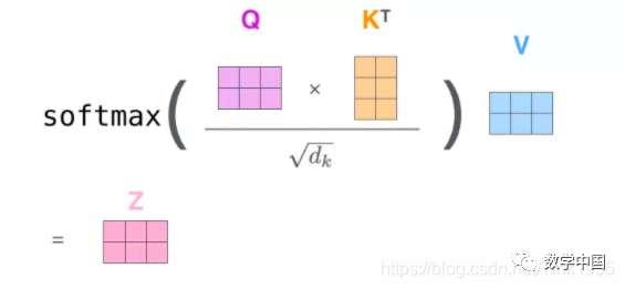
Step 3: Use the softmax function to convert the relevance score vector between each word into a probability distribution between [0,1], which emphasizes the relationships between words. After applying softmax, the score is transformed into a probability distribution matrix (2,2) α with values between [0,1].
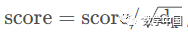
Step 4: Based on the probability distribution between each word, multiply by the corresponding Values, α and V are dot-multiplied: Z = softmax(score) ⋅ V, where V has a dimension of (2,64), and the final Z is a (2,64)-dimensional matrix.
The overall computation graph is as follows:
After discussing self-attention, what about Multi-Head Attention?
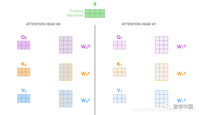
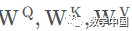
Multi-Head Attention is quite simple; it uses multiple sets of transformations to obtain Query, Keys, and Values from the input embedding matrix, rather than just one set as in self-attention.
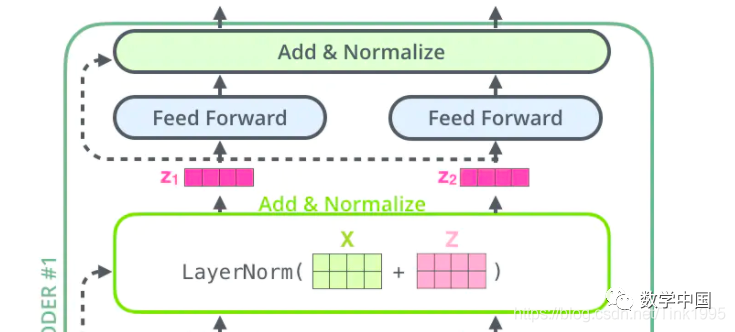
After obtaining the Z matrix from Multi-Head Attention, it is not directly passed to the fully connected neural network FNN, but goes through an additional step: Add & Normalize.
Add & Normalize:
Add
Add refers to the addition of a residual block X to Z. The purpose of adding the residual block X is to prevent degradation issues that can occur during training of deep neural networks. Degradation refers to the phenomenon where increasing the number of layers in a deep neural network leads to a gradual decrease in loss, stabilizing and saturating, and then further increasing the number of layers results in increased loss. You might have many questions about this! Why does degradation occur in deep neural networks, and how does adding a residual block prevent this issue? This involves knowledge of ResNet residual networks. Since this is a beginner-friendly series, I will explain every question clearly!
ResNet Residual Networks:
First, let’s address the question of why degradation occurs in deep neural networks.
For example, if the optimal number of layers for a neural network is 18, but we design it with 32 layers, then 14 of those layers are redundant. To achieve the optimal performance of an 18-layer network, we must ensure that these additional 14 layers perform identity mapping. Identity mapping means that the input equals the output, akin to F(x)=x. This ensures that the extra 14 layers do not affect the optimal performance.
However, in reality, the parameters of a neural network are learned, and ensuring that these parameters can accurately perform F(x)=x is quite difficult. A few redundant layers may not have a significant impact, but if the redundancy is too high, the results may not be ideal. At this point, experts proposed ResNet residual networks to address the degradation issue in neural networks.
What is a residual block?
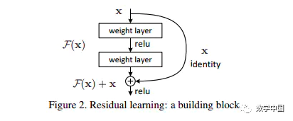
The above image shows a constructed residual block. Here, X is the input to this layer of the residual block, and F(X) is the residual output after the first linear transformation and activation. The diagram indicates that in a residual network, after the second layer undergoes linear transformation before activation, F(X) adds the input value X, and then the output is activated. This path is called a shortcut connection.
Why does adding a residual block prevent degradation issues in neural networks?
Let’s take a look at what the function looks like with the addition of a residual block. It changes to h(X)=F(X)+X. To achieve h(X)=X, we need F(X)=0. This is clever! It is much easier for a neural network to learn to become 0 than to learn to become X. As we know, neural network parameters are usually initialized as random numbers between [0,1]. So, after network transformations, it is easier to approach 0. For example:
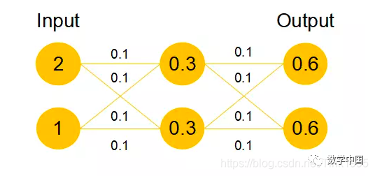
Assuming that this network undergoes only linear transformations, without bias or activation functions, we find that due to random initialization of weights, the output will be [0.6, 0.6], which is closer to [0, 0] than to [2, 1]. Thus, it is easier for the model to learn h(x)=x than F(x)=0. Moreover, ReLU can activate negative values to 0, filtering out negative linear transformations and speeding up the process of making F(x)=0. This allows the ResNet network to significantly mitigate the issue of learning identity mappings by updating the parameters of the redundant layers using the learned residual F(x)=0.
Thus, when the network decides which layers are redundant, it uses the learned residual F(x)=0 to ensure that the performance of the network with these redundant layers is equivalent to that of a network without them, significantly addressing the degradation issue.
Now that we have discussed why we need to add X and perform the shortcut in the residual network, do you understand?
Normalize
Why do we perform normalization?
Before training a neural network, we need to normalize the input data for two main reasons: 1) to speed up training, and 2) to improve training stability.
Why use Layer Normalization (LN) instead of Batch Normalization (BN)?
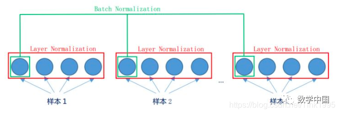
In the image, LN normalizes between different neurons within the same sample, while BN normalizes between the same position neurons across different samples in the same batch.
BN normalizes across the same dimension, but in NLP, the inputs are word vectors, and analyzing each dimension individually is meaningless. Therefore, normalization across each dimension is not suitable, which is why we choose LN.
Feed-Forward Networks
The formula for the fully connected layer is as follows:
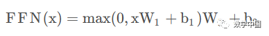
Here, the fully connected layer is a two-layer neural network, first undergoing linear transformation, then applying ReLU non-linearity, followed by another linear transformation.
In this case, x represents the output Z from Multi-Head Attention. Referring to the previous example, Z is a (2,64) dimensional matrix. Assuming W1 is (64,1024) and W2 is (1024,64), according to the formula:
FFN(Z)=(2,64)x(64,1024)x(1024,64)=(2,64). We notice that the dimensions remain unchanged; these two layers are intended to map the input Z into a higher-dimensional space (2,64)x(64,1024)=(2,1024), then return to the original dimension after applying the non-linear function.
After passing through Add & Normalize, the output enters the next encoder. After six encoders, it is sent to the decoder. Thus, we have completed the introduction of the Encoder section of the Transformer. Understanding the Encoder makes the Decoder quite easy; now let’s move on to the Decoder part!
2.3 Decoder of the Transformer
Looking at the Decoder block in the third part of the above image. The Decoder block also consists of six decoders stacked together, Nx=6. The gray box in part 3 of the image shows the internal structure of a decoder. From the diagram, we can see that a decoder is composed of Masked Multi-Head Attention, Multi-Head Attention, and a fully connected neural network FNN. The Decoder has an additional Masked Multi-Head Attention compared to the Encoder, while the other structures are similar, so let’s first look at this Masked Multi-Head Attention.
Input to the Transformer Decoder
The input to the Decoder is divided into two categories:
One is the input during training, and the other is the input during prediction.
The input during training consists of the corresponding target data that has been prepared. For example, in a translation task, the Encoder inputs “Tom chase Jerry,” while the Decoder inputs “汤姆追逐杰瑞.”
The input during prediction starts with the start token, and each subsequent input is the output of the previous time step of the Transformer. For example, input “”, output “汤姆”; input “汤姆”, output “汤姆追逐”; input “汤姆追逐”, output “汤姆追逐杰瑞”; input “汤姆追逐杰瑞”, output “汤姆追逐杰瑞” (end).
Masked Multi-Head Attention
The calculation principle of Masked Multi-Head Attention is the same as that of the Encoder’s Multi-Head Attention, but it adds a mask code. The mask indicates which values to hide so that they do not affect parameter updates. The Transformer model involves two types of masks: padding mask and sequence mask. Why do we need to add these two types of masks?
1. Padding Mask
What is a padding mask? Since the lengths of input sequences in each batch are different, we need to align the input sequences. Specifically, this means padding shorter sequences with 0 at the end. However, if an input sequence is too long, we truncate the left side and discard the excess. Since these padding positions are meaningless, our attention mechanism should not focus on them, so we need to process them.
The specific approach is to add a very large negative number (negative infinity) to these positions, so that after applying softmax, the probabilities for these positions will approach 0!
2. Sequence Mask
Sequence mask is used to ensure that the decoder cannot see future information. For a sequence, at time step t, the output of our decoding should only depend on the outputs before time t and not on those after time t. Therefore, we need a method to hide the information after t. This is effective during training because we input the complete target data into the decoder, but during prediction, we can only get the output predicted at the previous time step.
So how do we do this? It’s quite simple: we create an upper triangular matrix with all values above the diagonal set to 0. By applying this matrix to each sequence, we can achieve our goal.
It might have been forgotten to mention that the Multi-Head Attention in the Encoder also needs to be masked, but in the Encoder, only the padding mask is needed, while in the Decoder, both padding and sequence masks are required. Other than this difference in masks, everything else is the same as in the Encoder!
Add & Normalize is also the same as in the Encoder, and next comes the second Multi-Head Attention in the Decoder, which has a slight difference from the Encoder’s Multi-Head Attention.
Encoder-Decoder Based Multi-Head Attention
The Multi-Head Attention in the Encoder is based on Self-Attention, while the second Multi-Head Attention in the Decoder is based on Attention. Its input Query comes from the output of the Masked Multi-Head Attention, while Keys and Values come from the output of the last layer in the Encoder.
Those who are as detail-oriented as I am might wonder why there are two Multi-Head Attention layers in the Decoder?
My personal understanding is that the first Masked Multi-Head Attention is to capture the information from previously predicted outputs, effectively recording the relationships between inputs at the current time step. The second Multi-Head Attention is to derive the next time step’s output information based on the current input, representing the relationship between the current input and the feature vectors extracted from the Encoder.
After the second Multi-Head Attention, the Feed Forward Network is the same as in the Encoder, and the output proceeds to the next decoder. After passing through six layers of decoders, it reaches the final output layer.
2.4 Output of the Transformer

The output, as shown in the figure, first undergoes a linear transformation, then Softmax to obtain the probability distribution of the output, and finally, through a dictionary, the word corresponding to the highest probability is output as our predicted result.
2.5 Structure Summary
That’s it! The above is the entire structural principle of the Transformer. The Transformer truly deserves to be one of the most popular models in recent years, with many clever details. Understanding it requires considerable effort. I wonder if you have a clearer understanding of the structure of the Transformer after reading this?
3. Advantages and Disadvantages of Transformers
Although Transformers are excellent, they are not perfect and have some shortcomings. Next, I will introduce their advantages and disadvantages:
Advantages:
1. Good performance
2. Can be trained in parallel, fast speed
3. Effectively solves long-distance dependency issues
Disadvantages:
1. Completely based on self-attention, which loses some positional information between words. Although positional encoding has been added to address this issue, there are still optimization opportunities.
5. Conclusion
The Transformer is a highly promising model, and subsequent models like BERT and GPT have emerged from it, which are NLP powerhouses. There are still many areas for optimization. Currently, the application of NLP in industry is far less than in CV, but natural language is a crucial piece of information for the continuation of human civilization. Without written language, how can we reflect on the development history of our ancestors? Without language, how can human society operate harmoniously? Everything you see in images and hear in words is converted into understandable text information in your brain. Therefore, the prospects for NLP remain incredibly vast. This is the best of times; because NLP is still in the exploratory phase, it is not too late to start learning now. I will continue to write this beginner-friendly series, hoping that it can help those new to NLP.