What Is Neural Network Algorithm?

The hottest technology right now is definitely artificial intelligence.

The underlying model of artificial intelligence is the “neural network”. Many complex applications (like pattern recognition, automatic control) and advanced models (like deep learning) are based on it. To learn artificial intelligence, one must start with it.

What is a neural network? It seems that there is a lack of popular explanations online.

A couple of days ago, I read Michael Nielsen’s open-source textbook “Neural Networks and Deep Learning” and unexpectedly found that the explanation in it is very easy to understand. Below, I will introduce what a neural network is according to this book.

1. Perceptron

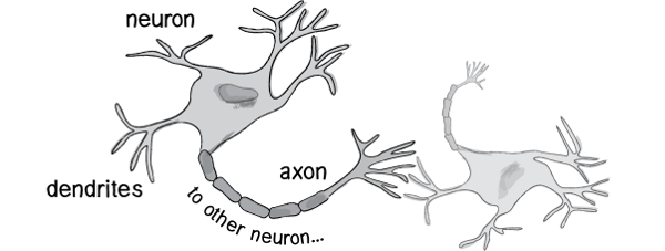
Historically, scientists have always hoped to simulate the human brain and create machines that can think. Why can humans think? Scientists have discovered that the reason lies in the human body’s neural network.

1. External stimuli are converted into electrical signals through nerve endings, which are transmitted to nerve cells (also called neurons).

2. Countless neurons make up the nerve center.

3. The nerve center integrates various signals and makes judgments.

4. The human body reacts to external stimuli based on the instructions from the nerve center.

Since the basis of thinking is neurons, if we could create “artificial neurons”, we could form an artificial neural network to simulate thinking. In the 1960s, the earliest model of “artificial neurons” was proposed, called the “perceptron”, which is still in use today.

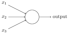
The circle in the above image represents a perceptron. It accepts multiple inputs (x1, x2, x3…), producing an output (output), similar to how nerve endings sense various changes in the external environment and finally generate electrical signals.

To simplify the model, we assume each input has only two possibilities: 1 or 0. If all inputs are 1, it indicates that all conditions are met, and the output is 1; if all inputs are 0, it indicates that none of the conditions are met, and the output is 0.

2. Example of Perceptron

Now let’s look at an example. The city is hosting an annual game and anime exhibition, and Xiao Ming is indecisive about whether to visit on the weekend.

He decides to consider three factors.

1. Weather: Is it sunny on the weekend?

2. Companions: Can he find someone to go with?

3. Price: Is the ticket affordable?

This forms a perceptron. The three factors above are the external inputs, and the final decision is the output of the perceptron. If all three factors are Yes (using 1 to indicate), the output is 1 (go visit); if all are No (using 0 to indicate), the output is 0 (do not go visit).

3. Weights and Thresholds

At this point, you may ask: What if some factors are met while others are not? For example, the weather is good, the ticket price is low, but Xiao Ming cannot find a companion; should he still go visit?

In reality, various factors rarely have equal importance: some factors are decisive, while others are secondary. Therefore, we can assign weights (weight) to these factors, representing their different levels of importance.

• Weather: weight of 8

• Companions: weight of 4

• Price: weight of 4

The weights above indicate that the weather is a decisive factor, while companions and price are secondary factors.

If all three factors are 1, their total weighted sum is 8 + 4 + 4 = 16. If the weather and price factors are 1, and the companion factor is 0, the total becomes 8 + 0 + 4 = 12.

At this point, we also need to specify a threshold (threshold). If the total is greater than the threshold, the perceptron outputs 1; otherwise, it outputs 0. Assuming the threshold is 8, then 12 > 8, and Xiao Ming decides to go visit. The height of the threshold represents the strength of the willingness; a lower threshold indicates a stronger desire to go, while a higher threshold indicates a weaker desire to go.

The decision process above can be expressed mathematically as follows.

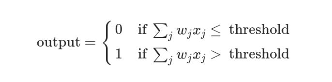
In the above formula, x represents various external factors, and w represents the corresponding weights.

4. Decision Model

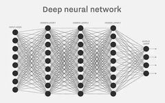
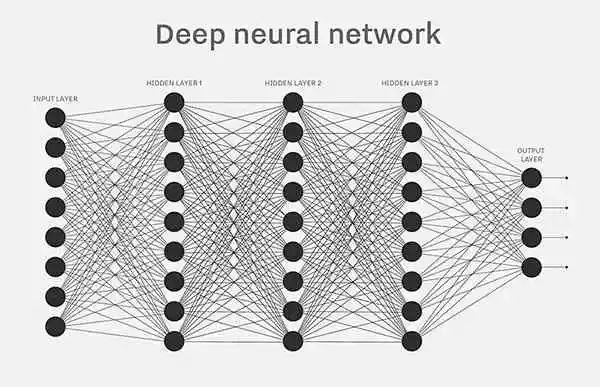
A single perceptron forms a simple decision model that can already be used. In the real world, actual decision models are much more complex, consisting of multiple perceptrons forming a multi-layer network.

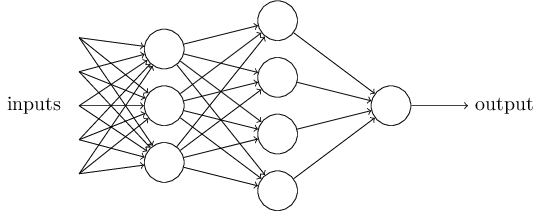
In the image above, the bottom layer perceptrons receive external inputs, make judgments, and then send signals as inputs to the upper layer perceptrons until the final result is obtained. (Note: The output of the perceptron still has only one, but it can be sent to multiple targets.)

In this diagram, the signals are all one-way, meaning that the output of the lower layer perceptrons is always the input of the upper layer perceptrons. In reality, there may be cyclic transmissions, meaning A sends to B, B sends to C, and C sends back to A; this is called a “recurrent neural network”, which is not covered in this article.

5. Vectorization

To facilitate further discussion, we need to perform some mathematical processing on the model above.

• External factors x1, x2, x3 are written as a vector , abbreviated as x

• Weights w1, w2, w3 are also written as a vector (w1, w2, w3), abbreviated as w

• Define the operation w⋅x = ∑ wx, which is the dot operation of w and x, equal to the sum of the products of factors and weights

• Define b as the negative threshold b = -threshold

The perceptron model then becomes as follows.

6. The Operation Process of Neural Networks

Building a neural network requires meeting three conditions.

• Input and output

• Weights (w) and thresholds (b)

• Structure of multi-layer perceptrons

In other words, we need to draw the diagram that has appeared above.

The most challenging part is determining the weights (w) and thresholds (b). So far, these two values are subjectively assigned, but it is very difficult to estimate their values in reality; a method is needed to find the answers.

This method is trial and error. Keeping all other parameters unchanged, a small change in w (or b) is noted as Δw (or Δb), and then the output is observed for any changes. This process is repeated until the corresponding w and b that yield the most accurate output are found; this process is called model training.

Therefore, the operation process of a neural network is as follows.

1. Determine input and output

2. Find one or more algorithms that can produce output from the input

3. Find a dataset with known answers to train the model and estimate w and b

4. Once new data is generated, input it into the model to obtain results while correcting w and b

As can be seen, the entire process requires massive computation. Therefore, neural networks have only become practically valuable in recent years, and standard CPUs are insufficient; specialized GPUs designed for machine learning are required for computation.

7. Example of Neural Networks

Now let’s explain neural networks through the example of automatic license plate recognition.

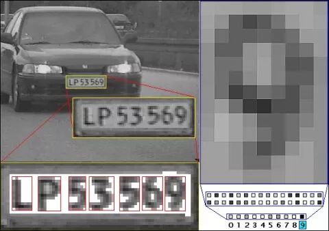
Automatic license plate recognition means that cameras on highways take photos of license plates, and computers recognize the numbers in the photos.

In this example, the license plate photo is the input, and the license plate number is the output. The clarity of the photo can set the weight (w). Then, find one or more image comparison algorithms to serve as the perceptron. The algorithm’s result is a probability, such as a 75% chance of determining it as the number 1. This requires setting a threshold (b) (for example, a confidence level of 85%); if it falls below this threshold, the result is invalid.

A set of already recognized license plate photos serves as training data, input into the model. By continuously adjusting various parameters, we find the combination that yields the highest accuracy. In the future, when new photos are received, results can be directly provided.

8. Continuity of Output

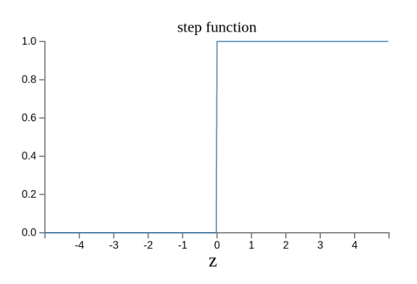
The model above has a problem that hasn’t been addressed: according to the assumption, the output only has two results: 0 and 1. However, the model requires that small changes in w or b will cause changes in output. If the output is only 0 and 1, it is too insensitive and cannot guarantee the correctness of training; therefore, the “output” must be transformed into a continuous function.

This requires a bit of simple mathematical modification.

First, we denote the calculation result of the perceptron wx + b as z.

z = wx + b

Then, calculate the following expression and denote the result as σ(z).

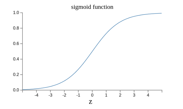
σ(z) = 1 / (1 + e^(-z))

This is because if z approaches positive infinity z → +∞ (indicating strong matching of the perceptron), then σ(z) → 1; if z approaches negative infinity z → -∞ (indicating strong mismatch of the perceptron), then σ(z) → 0. In other words, as long as σ(z) is used as the output result, the output will become a continuous function.

The original output curve looks like this.

Now it looks like this.

In fact, it can also be proven that Δσ satisfies the following formula.

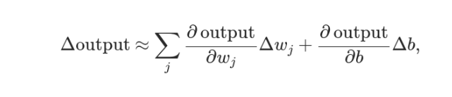
That is, the relationship between Δσ, Δw, and Δb is linear, and the rate of change is the partial derivative. This is beneficial for accurately calculating the values of w and b.

This article is reproduced from Ruan Yifeng’s blog.

– End –

What topics would you like to read about, dear friends?

Feel free to leave a message in the comment section.