Click on "Xiaobai Learns Vision" above, choose to add "Star" or "Top"
Heavy content delivered at the first time
Introduction
This article adopts an image presentation approach to help everyone understand the related complex mathematical equations. It focuses on understanding how neural networks work, mainly focusing on some typical issues of CNNs: the data structure of digital images, stride convolution, connection pruning and parameter sharing, backpropagation of convolutional layers, pooling layers, etc.
Original Title: Gentle Dive into Math Behind Convolutional Neural Networks
Fields such as autonomous driving, smart healthcare, and self-service retail were considered impossible until recently, and computer vision has helped us achieve these things. Today, the dream of having autonomous vehicles or automated grocery stores no longer sounds so unattainable. In fact, we use computer vision every day—when we unlock our phones with facial recognition or use auto-enhance before posting photos on social media. Convolutional neural networks may be the most critical building blocks behind this tremendous success. This time, we will deepen our understanding of how neural networks work with CNNs. As a suggestion, this article will include quite complex mathematical equations, so if you are not familiar with linear algebra and calculus, please do not be discouraged. My goal is not to make you memorize these formulas but to give you an intuitive understanding of what is happening below.
Note: In this article, I mainly focus on some typical issues of CNNs. If you are looking for more basic information about deep neural networks, I suggest you read my other articles in this series (https://towardsdatascience.com/https-medium-com-piotr-skalski92-deep-dive-into-deep-networks-math-17660bc376ba). As always, you can find the complete source code with visualizations and annotations on my GitHub (https://github.com/SkalskiP/ILearnDeepLearning.py). Let’s get started!
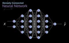
In the past, we already knew about neural networks known as dense connections. The neurons of these networks are divided into several groups, forming continuous layers. Each such neuron is connected to every neuron in the adjacent layer. The figure below shows an example of this architecture.
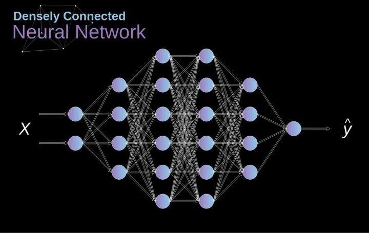 Figure 1. Structure of Dense Connected Neural Networks
When we solve classification problems based on a set of limited manually designed features, this method works effectively. For example, we predict a soccer player’s position based on his statistics during a match. However, the situation becomes more complex when dealing with photos. Of course, we can treat the pixel values of each pixel as individual features and pass them as inputs to our dense network. Unfortunately, to make this network applicable to a specific smartphone photo, our network would need to contain tens of millions or even hundreds of millions of neurons. On the other hand, we could downscale our photos, but in the process, we would lose some useful information. We immediately realize that traditional strategies do not work for us; we need a new effective method to make the most of as much data as possible while reducing the required computation and parameter count. This is where CNNs come into play.
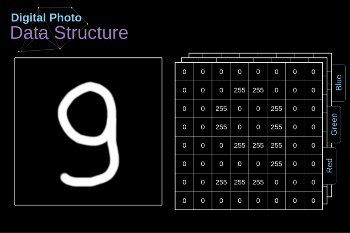
Let’s take some time to explain how digital images are stored. Most of you may know that they are actually a matrix composed of many numbers. Each of these numbers corresponds to the brightness of a pixel. In the RGB model, a color image is actually composed of three matrices corresponding to the red, green, and blue color channels. In black and white images, we only need one matrix. Each matrix stores values between 0 and 255. This range is a compromise between the efficiency of storing image information (values within 256 can be expressed using one byte) and the sensitivity of the human eye (we can distinguish a limited number of identical color grayscale values).
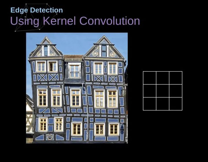
Convolution is not only used in neural networks but is also a key component of many other computer vision algorithms. In this process, we take a smaller-shaped matrix (called a kernel or filter), input the image, and transform the image based on the values of the filter. The subsequent feature map values are calculated using the following formula, where the input image is represented by f, our kernel by h, and the row and column indices of the result matrix are represented by m and n, respectively.

After placing the filter on the selected pixel, we extract the values from the kernel at each corresponding position and multiply them with the corresponding values in the image. Finally, we summarize everything and place the result in the corresponding position of the output feature map. Above, we can see how such an operation is implemented in detail, but what is more concerning is what applications we can achieve by performing kernel convolution over a complete image. Figure 4 shows the convolution results of several different filters.
As shown in Figure 3, when we convolve a 6×6 image with a 3×3 kernel, we get a 4×4 feature map. This is because there are only 16 different positions where we can place the filter in this image. Because each convolution operation reduces the size of the image, we can only perform a limited number of convolutions until the image completely disappears. More importantly, if we observe how the convolution kernel moves within the image, we will find that the influence of pixels located at the edges of the image is much smaller than that of pixels located at the center of the image. Thus, we lose some information contained in the image. The following diagram shows how the position of pixels changes its influence on the feature map.
To solve these two problems, we can pad the image with an extra border. For example, if we use a 1px padding, we increase the size of the photo to 8×8, then the output of convolving with a 3×3 filter will be 6×6. In practice, we usually use 0 padding for the extra padding area. Depending on whether we use padding, we will judge based on two types of convolution—valid convolution and same convolution. This naming is not very appropriate, so for clarity: Valid means we only use the original image, Same means we also consider the surrounding border of the original image, so the input and output image sizes are the same. In the second case, the padding width should satisfy the following equation, where p is the padding width and f is the filter dimension (generally odd).


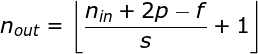
In the previous example, we always moved the convolution kernel one pixel at a time. However, stride can also be considered as one of the hyperparameters of the convolution layer. In Figure 6, we can see what the convolution looks like if we use a larger stride. When designing the CNN architecture, if we want less overlap in the receptive field, or if we want the spatial dimensions of the feature map to be smaller, we can decide to increase the stride. The size of the output matrix—considering padding width and stride—can be calculated using the following formula.
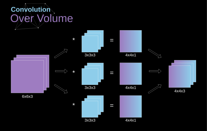
Spatial convolution is a very important concept that allows us to process color images and, more importantly, to apply multiple convolution kernels in a single layer. The first important principle is that the filter and the image to which it is applied must have the same number of channels. Essentially, this way is very similar to the example in Figure 3, but this time we multiply the values in three-dimensional space with the corresponding convolution kernels. If we want to use multiple filters on the same image, we convolve them separately, stack the results, and combine them into a whole. The dimensions of the receiving tensor (i.e., our three-dimensional matrix) satisfy the following equation: n – image size, f – filter size, nc – number of channels in the image, p – whether padding is used, s – stride used, nf – number of filters.

Now it’s time to apply the knowledge we learned today to construct our CNN layers. Our approach is almost the same as the one we used in dense connected neural networks, with the only difference being that this time we will use convolution instead of simple matrix multiplication. Forward propagation consists of two steps. The first step is to calculate the intermediate value Z, which is obtained by convolving the input data and the weight tensor W from the previous layer (including all filters), and then adding the bias b. The second step is to apply the nonlinear activation function to the obtained intermediate value (our activation function is represented as g). Readers interested in the matrix equation can find the corresponding mathematical formulas below. If you are unclear about the operational details, I strongly recommend my previous article, in which I discuss the principles of dense connected neural networks in detail. By the way, in the diagram below, you can see a simple visualization describing the dimensions of the tensors used in the equation.

Connection Pruning and Parameter Sharing
At the beginning of the article, I mentioned that dense connected neural networks are not good at processing images because they require learning a large number of parameters. Now that we understand what convolution is, let’s consider how it optimizes computation. In the diagram below, the two-dimensional convolution is displayed in a slightly different way, with the neurons marked with numbers 1-9 forming the input layer and receiving the pixel brightness values of the image, while units A – D represent the computed feature map elements. Finally, I-IV are the values of the convolution kernels that need to be learned.
Now, let’s focus on two very important properties of the convolution layer. First, you can see that not all neurons in consecutive layers are connected to each other. For example, neuron 1 only affects the value of A. Secondly, we see that some neurons share the same weights. These two properties mean that we need to learn far fewer parameters. By the way, it is worth noting that one value in the filter affects every element in the feature map—this is very important in the backpropagation process.
Backpropagation of Convolutional Layers
Anyone who has tried to write their own neural network code from scratch knows that completing forward propagation does not complete half of the algorithm process. The real fun comes when you want to perform backpropagation. Now, we don’t need to be troubled by the issue of backpropagation; we can utilize deep learning frameworks to implement this part, but I think it is valuable to understand the underlying principles. Just like in dense connected neural networks, our goal is to compute the derivatives and then use them to update our parameter values—this process is called gradient descent.
In our calculations, we need to use the chain rule—which I mentioned in previous articles. We want to evaluate how changes in parameters affect the final feature map and subsequently the final result. Before we start discussing the details, let’s unify the mathematical symbols used—so as to simplify the process, I will abandon the full notation of partial derivatives and use a shorter notation as shown below. But remember, when I use this notation, I always refer to the partial derivative of the loss function.

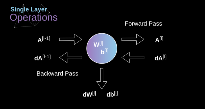
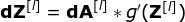
Our task is to compute dW[l] and db[l]—which are the derivatives related to the current layer parameters, as well as the value of dA[l -1]—which will be passed to the previous layer. As shown in Figure 10, we receive dA[l] as input. Of course, the dimensions of tensors dW and W, db and b, and dA and A are the same. The first step is to obtain the intermediate value dZ[l] by taking the derivative of the activation function of the input tensor. According to the chain rule, the results obtained from this operation will be used later.
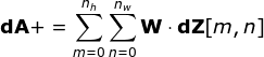
Now, we need to deal with the backpropagation of the convolution itself. To achieve this, we will use a matrix operation called full convolution, as shown in the figure below. Note that in this process, we rotate the convolution kernel 180 degrees. This operation can be described using the following formula, where the filter is represented by W, and dZ[m,n] is a scalar belonging to the partial derivative of the previous layer.
In addition to convolution layers, CNNs also frequently use so-called pooling layers. Pooling layers are mainly used to reduce the size of tensors and speed up computation. This network layer is straightforward—we need to segment the image into different regions and then perform some operations on each part. For example, for a max pooling layer, we select the maximum value from each region and place it in the corresponding position in the output. In the case of convolution layers, we have two hyperparameters—the filter size and the stride. One last important point is that if pooling operations are to be performed on multi-channel images, they should be performed separately for each channel.
In this article, we will only discuss the backpropagation of max pooling, but the rules we learn can be applied to all types of pooling layers with slight adjustments. Since there are no parameters to update in this type of layer, our task is simply to distribute the gradients appropriately. As we remember, in the forward propagation of max pooling, we select the maximum value from each region and pass them to the next layer. Therefore, it is clear that during backpropagation, gradients should not affect elements in the matrix that were not included in the forward propagation. In fact, this is achieved by creating a mask that remembers the positions of the values used in the first phase, which we can later use to propagate the gradients.
Congratulations on making it here. Thank you very much for taking the time to read this article. If you liked this post, you might consider sharing it with your friends, or two or five friends. If you notice any incorrect thinking, formulas, animations, or code, please let me know.
This article is another part of the “Mysteries of Neural Networks” series. If you haven’t had the chance to read the other articles, please check them out (https://towardsdatascience.com/preventing-deep-neural-network-from-overfitting-953458db800a). Also, if you like the work I do, follow me on Twitter and Medium, and check out other projects I’m working on, like GitHub (https://github.com/SkalskiP) and Kaggle (https://www.kaggle.com/skalskip). Stay curious!
via: https://towardsdatascience.com/gentle-dive-into-math-behind-convolutional-neural-networks-79a07dd44cf9
Good news!
Xiaobai Learns Vision Knowledge Planet
is now open to the public👇👇👇


Download 1: OpenCV-Contrib Extension Module Chinese Version Tutorial
Reply "Extension Module Chinese Tutorial" in the backend of "Xiaobai Learns Vision" WeChat public account to download the first OpenCV extension module tutorial in Chinese on the internet, covering more than twenty chapters including extension module installation, SFM algorithms, stereo vision, target tracking, biological vision, super-resolution processing, etc.

Download 2: 52 Lectures on Python Vision Practical Projects
Reply "Python Vision Practical Projects" in the backend of "Xiaobai Learns Vision" WeChat public account to download 31 practical vision projects including image segmentation, mask detection, lane line detection, vehicle counting, eye line addition, license plate recognition, character recognition, emotion detection, text content extraction, face recognition, etc., to help quickly learn computer vision.

Download 3: 20 Lectures on OpenCV Practical Projects
Reply "OpenCV Practical Projects 20 Lectures" in the backend of "Xiaobai Learns Vision" WeChat public account to download 20 practical projects based on OpenCV to achieve advanced learning of OpenCV.

Discussion Group

Welcome to join the reader group of the public account to communicate with peers. Currently, there are WeChat groups for SLAM, 3D vision, sensors, autonomous driving, computational photography, detection, segmentation, recognition, medical imaging, GAN, algorithm competitions, etc. (will be gradually subdivided in the future). Please scan the WeChat number below to join the group, and note: "Nickname + School/Company + Research Direction", for example: "Zhang San + Shanghai Jiao Tong University + Vision SLAM". Please follow the format for remarks; otherwise, you will not be approved. After successful addition, you will be invited to enter the relevant WeChat group based on your research direction. Please do not send advertisements in the group; otherwise, you will be removed from the group. Thank you for your understanding~