Source: Python Data Science


This article is approximately 7200 words long and is recommended to be read in 14 minutes.
In this article, we will explore the Transformer model and understand how it works.
1. Introduction
The BERT model launched by Google achieved SOTA results in 11 NLP tasks, igniting the entire NLP community. One key factor in BERT’s success is the powerful role of the Transformer. The Google Transformer model was initially used for machine translation tasks, achieving SOTA results at that time. The Transformer improved the slow training issue commonly criticized in RNNs by utilizing the self-attention mechanism for fast parallel processing. Additionally, the Transformer can scale to very deep depths, fully exploiting the characteristics of DNN models and enhancing model accuracy. In this article, we will study the Transformer model and understand how it works.
2. Main Content Begins
The Transformer was proposed in the paper “Attention is All You Need” and is now the recommended reference model for Google Cloud TPU. The TensorFlow code related to the paper can be obtained from GitHub as part of the Tensor2Tensor package. Harvard’s NLP team has also implemented a PyTorch-based version with annotations of the paper.
In this article, we will attempt to simplify the model a bit and introduce the core concepts one by one, hoping to make it easy for ordinary readers to understand.
Attention is All You Need:
https://arxiv.org/abs/1706.03762
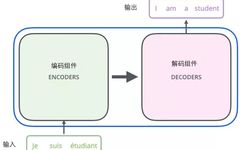
Starting from a macroscopic perspective, we can view this model as a black box operation. In machine translation, it means inputting one language and outputting another.

By breaking down this black box, we can see that it consists of an encoding component, a decoding component, and the connections between them.
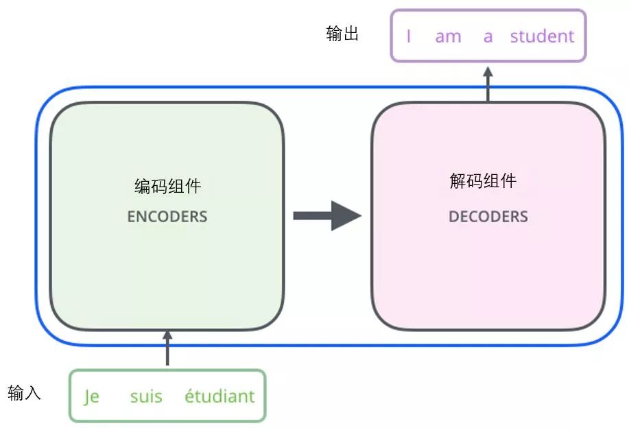
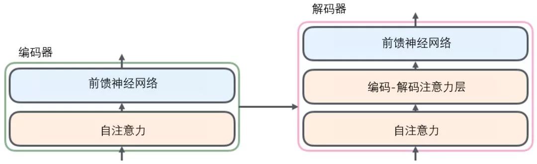
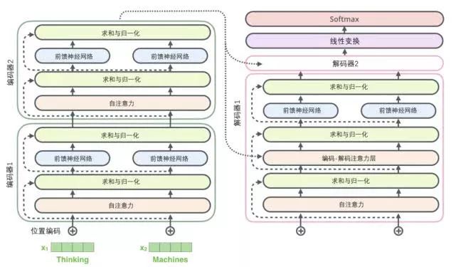
The encoding component consists of a stack of encoders (the paper stacks 6 encoders together — the number 6 is not magical; you can try other numbers). The decoding component also consists of the same number (corresponding to the encoders) of decoders.
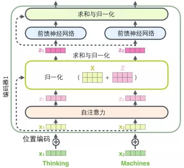
All encoders are structurally identical, but they do not share parameters. Each decoder can be decomposed into two sub-layers.
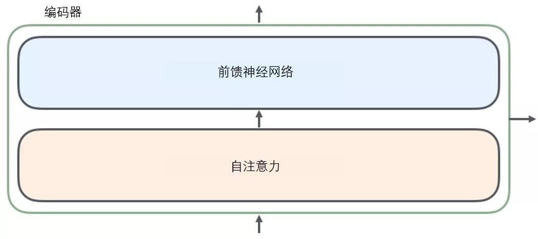
The sentence input from the encoder first passes through a self-attention layer, which helps the encoder focus on other words in the input sentence while encoding each word. We will delve deeper into self-attention later in the article.
The output of the self-attention layer is passed to a feed-forward neural network. The feed-forward neural network corresponding to each position’s word is identical (another interpretation is a one-dimensional convolutional neural network with a window size of one word).
The decoder also has the encoder’s self-attention layer and feed-forward layer. Additionally, there is an attention layer between these two layers to focus on relevant parts of the input sentence (similar to the attention mechanism in seq2seq models).
Introducing Tensors
We have understood the main parts of the model; next, let’s look at how various vectors or tensors (note: the concept of a tensor is a generalization of the concept of a vector; you can simply understand that a vector is a first-order tensor, and a matrix is a second-order tensor) transform the input into output in different parts of the model.
Like most NLP applications, we first convert each input word into a word vector using a word embedding algorithm.
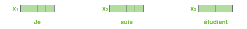
Each word is embedded as a 512-dimensional vector, and we use these simple boxes to represent these vectors.
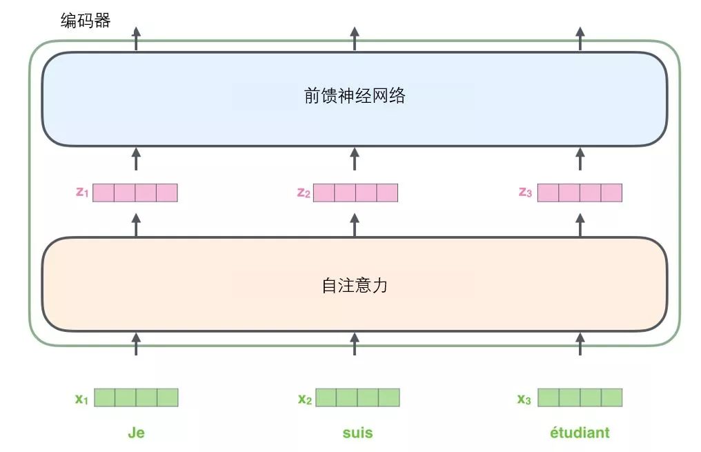
The word embedding process occurs only in the bottommost encoder. All encoders share a common feature: they receive a list of vectors, each of which has a size of 512 dimensions. In the bottom (initial) encoder, it is the word vectors, but in other encoders, it is the output of the next layer encoder (also a list of vectors). The size of the vector list is a hyperparameter that we can set — generally, it is the length of the longest sentence in our training set.
After embedding the input sequence, each word will flow through the two sub-layers in the encoder.
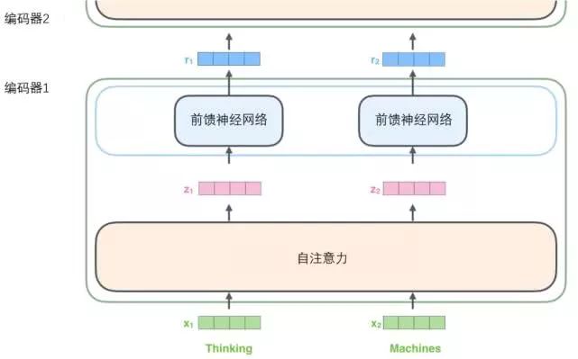
Next, let’s look at a core feature of the Transformer; here, each word at each position in the input sequence has its unique path flowing into the encoder. In the self-attention layer, there are dependencies between these paths. However, the feed-forward layer does not have these dependencies. Thus, various paths can be executed in parallel during the feed-forward layer.
Then we will take a shorter sentence as an example to see what happens in each sub-layer of the encoder.
Now We Begin to “Encode”
As mentioned above, an encoder receives a list of vectors as input, then passes the vectors in the list to the self-attention layer for processing, and then passes the output to the feed-forward neural network layer, which sends the results to the next encoder.
Each word in the input sequence undergoes a self-encoding process. Then, they each pass through the same feed-forward neural network, while each vector goes through it separately.
Macroscopic View of the Self-Attention Mechanism
Don’t be confused by the term self-attention, as if everyone should be familiar with this concept. In fact, I hadn’t encountered this concept until I read the paper Attention is All You Need. Let’s clarify how it works.
For example, the following sentence is our input sentence we want to translate:
The animal didn’t cross the street because it was too tired
What does “it” refer to in this sentence? Does it refer to the street or the animal? This is a simple question for humans, but not for algorithms.
When the model processes the word “it,” the self-attention mechanism allows “it” to establish a connection with “animal.”
As the model processes each word in the input sequence, self-attention attends to all words in the input sequence, helping the model encode the current word better.
If you are familiar with RNNs (Recurrent Neural Networks), recall how it maintains the hidden layer. RNNs combine the representations of all previously processed words/vectors with the current word/vector being processed. The self-attention mechanism incorporates the understanding of all relevant words into the word we are currently processing.
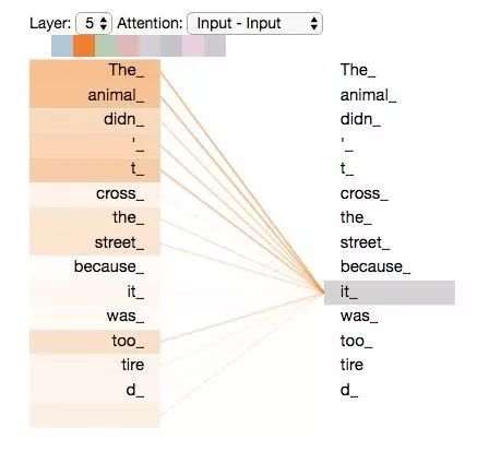 When we encode the word “it” in encoder #5 (the topmost encoder in the stack), the attention mechanism will focus on “The Animal,” incorporating part of its representation into the encoding of “it.”
Be sure to check the Tensor2Tensor notebook, where you can download a Transformer model and interactively visualize it.
Microscopic View of the Self-Attention Mechanism
First, let’s understand how to calculate self-attention using vectors, and then see how it is implemented using matrices.
The first step in calculating self-attention is to generate three vectors from each encoder’s input vector (the word vector for each word). In other words, for each word, we create a query vector, a key vector, and a value vector. These three vectors are created by multiplying the word embedding with three weight matrices.
It can be observed that these new vectors are lower in dimension than the word embedding vectors. Their dimension is 64, while the dimensions of the word embedding and the input/output vectors of the encoder are 512. However, it is not strictly required for the dimensions to be smaller; this is just an architectural choice that keeps most of the calculations of multi-headed attention invariant.
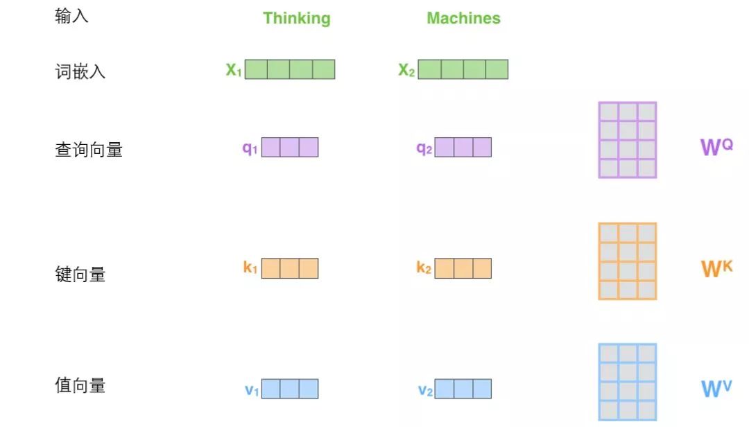
X1 multiplied by the WQ weight matrix gives q1, which is the query vector associated with this word. Ultimately, each word in the input sequence creates a query vector, a key vector, and a value vector.
What are Query Vectors, Key Vectors, and Value Vectors?
They are all abstract concepts that help compute and understand the attention mechanism. Please continue reading the content below to find out what role each vector plays in calculating the attention mechanism.
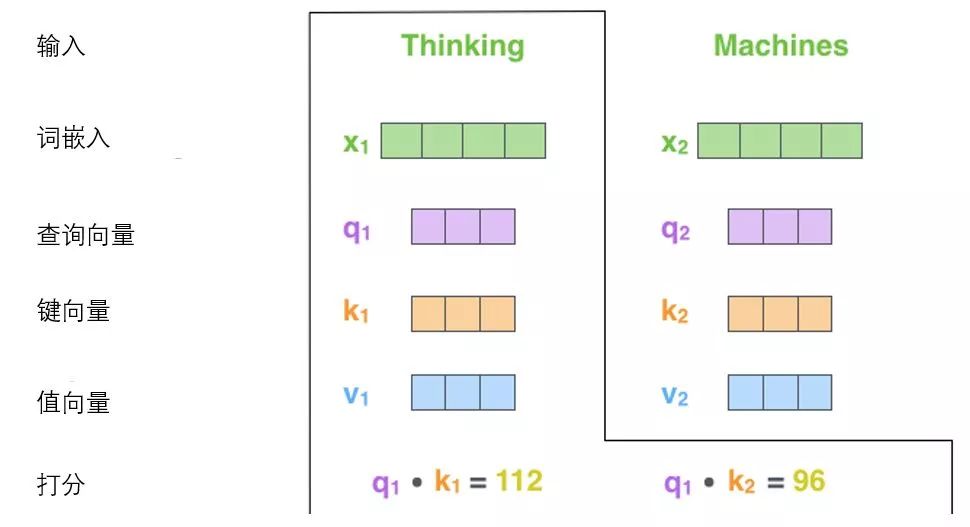
The second step in calculating self-attention is to compute the scores. Suppose we are calculating the self-attention vector for the first word “Thinking” in this example; we need to score each word in the input sentence against “Thinking.” These scores determine how much emphasis is placed on other parts of the sentence when encoding the word “Thinking.”
These scores are calculated by taking the dot product of the key vectors of the scored words (all words in the input sentence) with the query vector of “Thinking.” So if we are processing the self-attention of the word in the first position, the first score is the dot product of q1 and k1, and the second score is the dot product of q1 and k2.
The third and fourth steps involve dividing the scores by 8 (8 is the square root of the dimensionality of the key vectors, which is 64, to stabilize the gradients. Other values can also be used; 8 is just the default value), and then passing the results through softmax. The role of softmax is to normalize the scores of all words, resulting in positive values that sum to 1.
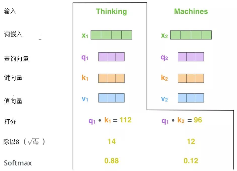
This softmax score determines each word’s contribution to the encoding of the current position (“Thinking”). Clearly, words already present at this position will receive the highest softmax scores, but sometimes it can also be beneficial to pay attention to another semantically related word.
The fifth step is to multiply each value vector by the softmax scores (this prepares them for summation later). The intuition here is to focus on semantically relevant words while downplaying irrelevant words (for example, multiplying them by a small decimal like 0.001).
The sixth step is to sum the weighted value vectors (note: another interpretation of self-attention is that when encoding a word, it is the weighted sum of all word representations (value vectors), where the weights are obtained through the dot product of the word’s representation (key vector) and the representation of the word being encoded (query vector)), and thus we obtain the output of the self-attention layer at that position (in our example, it is for the first word).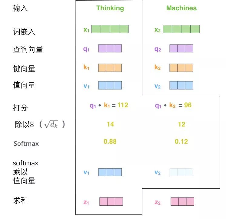
Thus, the calculation of self-attention is complete. The resulting vector can then be passed to the feed-forward neural network. However, in practice, these calculations are done in matrix form to speed up computation. Next, let’s see how this is implemented using matrices.
Implementing Self-Attention Mechanism via Matrix Operations
The first step is to compute the query matrix, key matrix, and value matrix. To do this, we pack the word embeddings of the input sentence into matrix X and multiply them by our trained weight matrices (WQ, WK, WV).
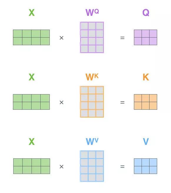
Each row in the x matrix corresponds to a word in the input sentence. We again see the size differences between the word embedding vectors (512, or the 4 boxes in the image) and the q/k/v vectors (64, or the 3 boxes in the image).
Finally, since we are dealing with matrices, we can combine steps 2 to 6 into a single formula to compute the output of the self-attention layer. Matrix Operation Form of Self-Attention
“The Battle of Multi-Headed Attention”
By adding a mechanism called “multi-headed attention,” the paper further improves the self-attention layer and enhances its performance in two aspects:
1. It expands the model’s ability to focus on different positions. In the above example, although each encoding has some representation in z1, it may be dominated by the actual words themselves. If we translate a sentence like “The animal didn’t cross the street because it was too tired,” we would want to know which word “it” refers to, and this is where the model’s “multi-head” attention mechanism comes into play.
2. It provides multiple “representation subspaces” for the attention layer. Next, we will see that for the “multi-headed” attention mechanism, we have multiple sets of query/key/value weight matrices (the Transformer uses eight attention heads, so we have eight sets of matrices for each encoder/decoder). Each of these sets is randomly initialized, and after training, each set is used to project the input word embeddings (or vectors from lower encoders/decoders) into different representation subspaces.
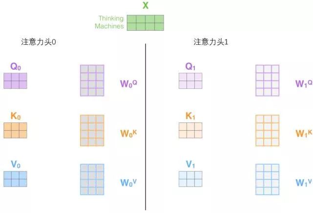
In the “multi-headed” attention mechanism, we maintain independent query/key/value weight matrices for each head, resulting in different query/key/value matrices. As before, we multiply X by the WQ/WK/WV matrices to produce the query/key/value matrices.
If we perform the same self-attention calculations as above, using eight different weight matrix operations, we will obtain eight different Z matrices.
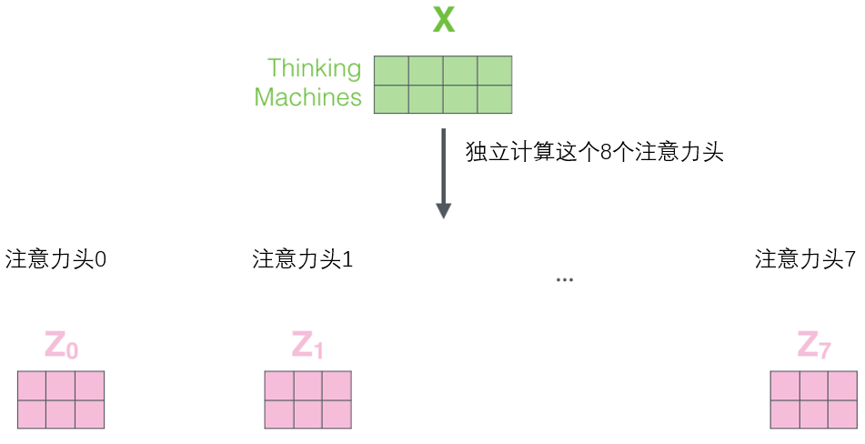
This presents us with a challenge. The feed-forward layer does not need eight matrices; it only requires one matrix (composed of the representation vectors of each word). So we need a way to compress these eight matrices into one matrix. How do we do this? We can concatenate these matrices together and then multiply them by an additional weight matrix WO.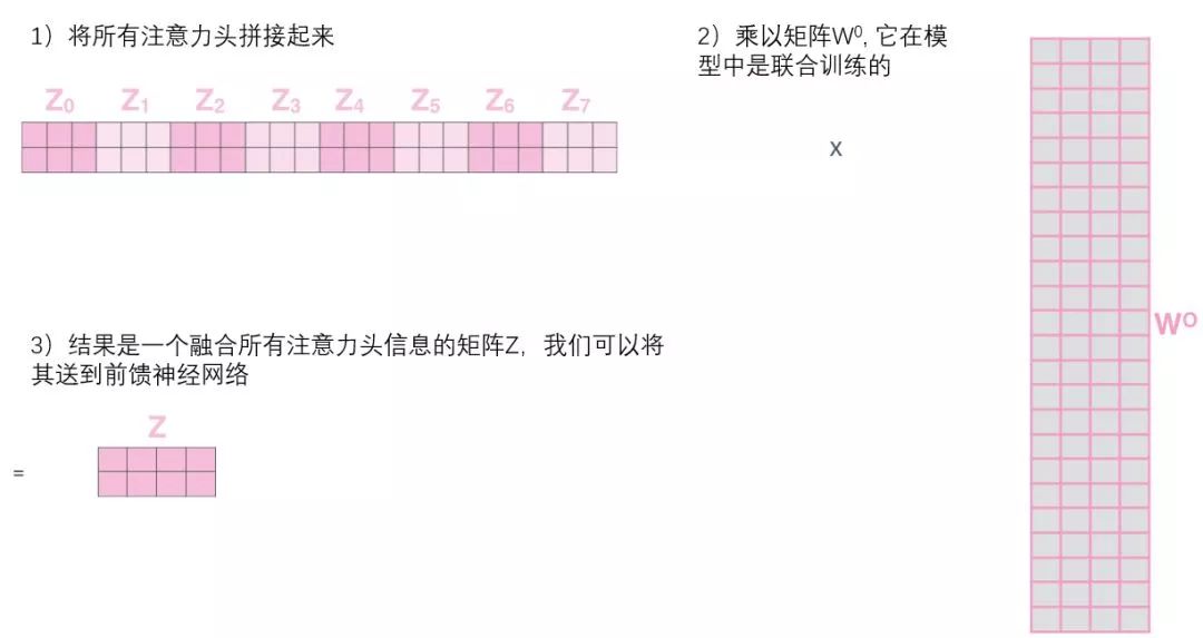
This is almost everything about multi-headed self-attention. There are indeed many matrices, and we try to consolidate them into one image for clarity.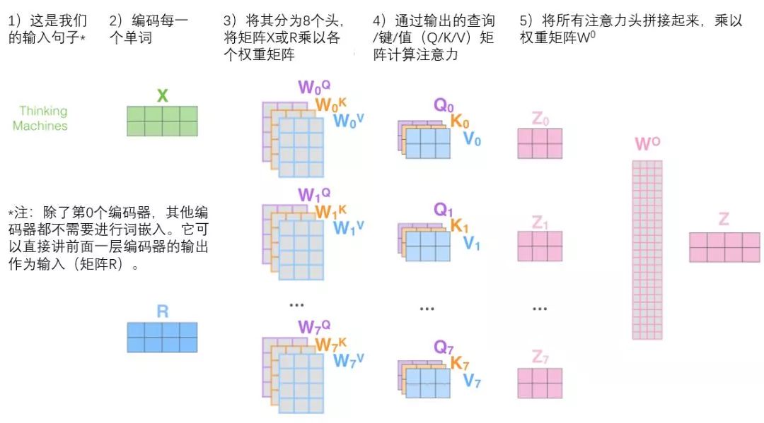
Now that we have grasped so many “heads” of the attention mechanism, let’s revisit the earlier example to see where different attention “heads” focus when encoding the word “it”: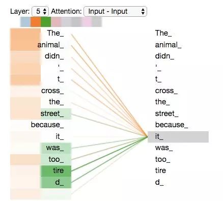
When we encode the word “it,” one attention head focuses on “animal,” while another focuses on “tired.” In a sense, the model’s representation of the word “it” is somewhat a combination of “animal” and “tired.”
However, if we add all the attention to the illustration, it becomes even harder to explain: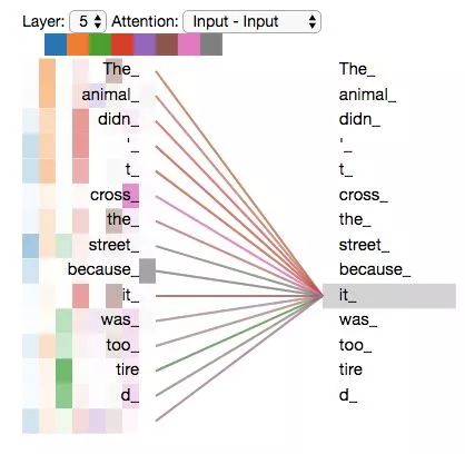
Using Positional Encoding to Represent Sequence Order
So far, our description of the model lacks a way to understand the order of input words.
To address this, the Transformer adds a vector for each input word embedding. These vectors follow a specific pattern learned by the model, which helps determine each word’s position or the distance between different words in the sequence. The intuition here is that adding position vectors to word embeddings allows them to better express the distances between words in subsequent operations.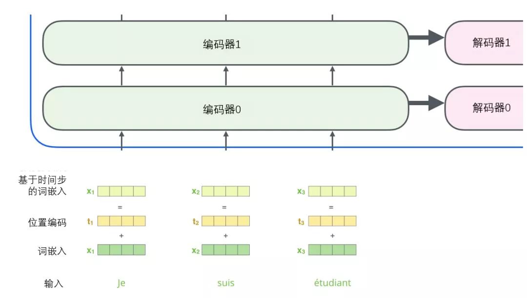
To help the model understand the order of words, we add positional encoding vectors, whose values follow a specific pattern.
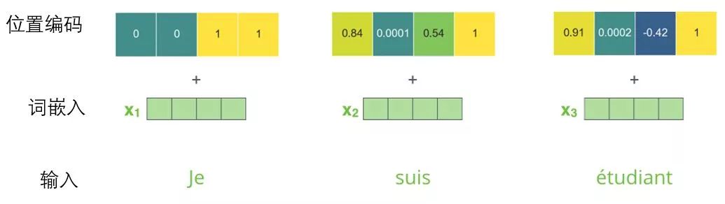
Mini word embedding positional encoding example with a size of 4
What would the pattern look like?
In the image below, each row corresponds to the positional encoding of a word vector, so the first row corresponds to the first word in the input sequence. Each row contains 512 values, each ranging between 1 and -1. We have color-coded them so that the pattern is visible.
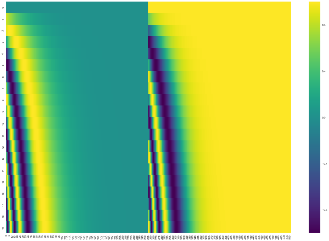
Example of positional encoding for 20 words (rows), with a word embedding size of 512 (columns). You can see it splits in the middle. This is because the values of the left half are generated by one function (using sine), while the right half is generated by another function (using cosine). They are then concatenated to obtain each positional encoding vector.
The original paper describes the formula for positional encoding (section 3.5). You can see the code for generating positional encodings in get_timing_signal_1d(). This is not the only possible method for positional encoding. However, its advantage is that it can scale to unknown sequence lengths (for example, when the trained model needs to translate sentences longer than those in the training set).
Residual Modules
Before we proceed, we need to mention a detail in the encoder architecture: there is a residual connection around each sub-layer (self-attention, feed-forward network) in each encoder, followed by a “layer normalization” step.
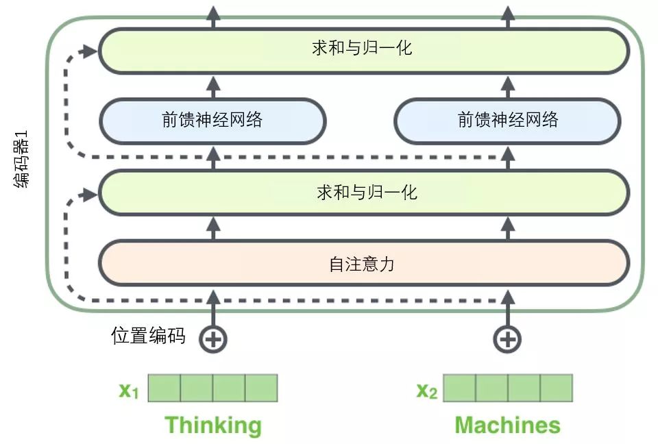
If we visualize these vectors along with the layer normalization operation associated with self-attention, it looks like the following figure describes:
The sub-layers of the decoder are similar. If we imagine a 2-layer encoder-decoder structure of the transformer, it would look like the following image:
 Decoder Component
Now that we have discussed most of the concepts of the encoder, we basically know how the decoder works. However, it’s best to look at the details of the decoder.
The encoder starts working by processing the input sequence. The output of the top encoder is then transformed into a set of attention vectors containing vectors K (key vectors) and V (value vectors). These vectors will be used by each decoder for its “encoder-decoder attention layer,” which helps the decoder focus on the appropriate positions in the input sequence:
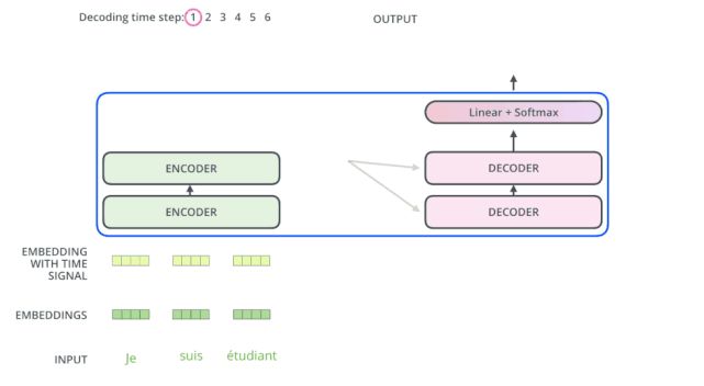
After completing the encoding phase, the decoding phase begins. Each step of the decoding phase outputs an element of the output sequence (in this example, the English translation of the sentence).
The subsequent steps repeat this process until a special termination symbol is reached, indicating that the transformer’s decoder has completed its output. The output at each step is provided to the bottom decoder at the next time step, and just as the encoders did before, these decoders will output their decoding results. Additionally, just like we did for the input to the encoder, we will embed and add positional encoding to those decoders to represent the position of each word.
The self-attention layers in those decoders behave differently from those in encoders: in the decoder, the self-attention layer is only allowed to process those positions in the output sequence that are further ahead. Before the softmax step, it will mask the later positions (setting them to -inf).
The “encoder-decoder attention layer” works similarly to the multi-headed self-attention layer, except that it creates the query matrix from the layers below it and retrieves the key/value matrices from the encoder’s output.
Final Linear Transformation and Softmax Layer
The decoder component will ultimately output a real-valued vector. How do we turn these floating-point numbers into a word? This is the job of the linear transformation layer, followed by the Softmax layer.
The linear transformation layer is a simple fully connected neural network that can project the vector produced by the decoder component into a much larger vector called logits.
Let’s assume our model learns 10,000 different English words from the training set (our model’s “output vocabulary”). Thus, the logits vector is a vector of length 10,000, where each cell corresponds to the score of a specific word.
The subsequent Softmax layer converts those scores into probabilities (all positive, with a maximum of 1.0). The cell with the highest probability is selected, and the corresponding word is output as the result for that time step.
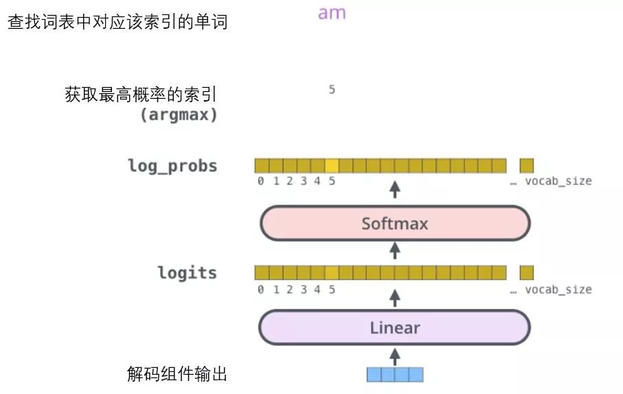 This image starts from the output vector produced by the decoder component. It then transforms it into an output word.
Summary of the Training Phase
Now that we have gone through the complete forward propagation process of the transformer, we can intuitively feel its training process.
During training, an untrained model goes through exactly the same forward propagation. However, because we train it using a labeled training set, we can compare its output with the actual output.
To visualize this process, let’s assume our output vocabulary only contains six words: “a,” “am,” “i,” “thanks,” “student,” and “” (the abbreviation for end of sentence).
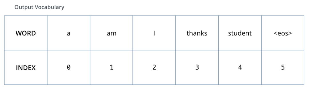
The output vocabulary of our model is set during the preprocessing phase before training.
Once we define our output vocabulary, we can use a vector of the same width to represent each word in our vocabulary. This is also known as one-hot encoding. So, we can represent the word “am” with the following vector:
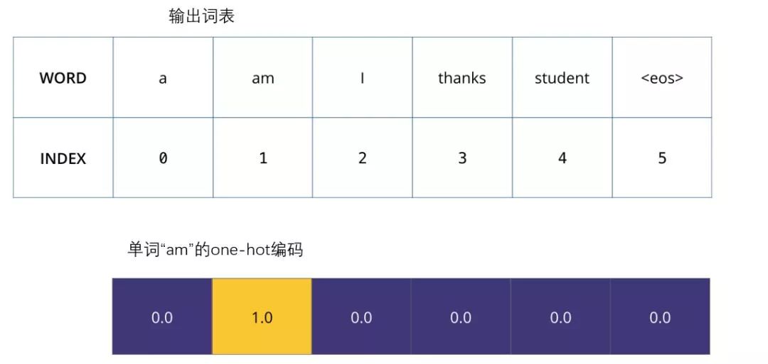
Example: One-hot encoding for our output vocabulary
Next, we discuss the model’s loss function — this is the criterion we optimize during training. It helps train a model that produces results as accurately as possible.
Loss Function
For instance, we are training the model, and now it’s the first step, a simple example — translating “merci” to “thanks.”
This means we want an output that represents the probability distribution of the word “thanks.” However, since this model is not yet trained, it is unlikely to produce this result at this time.
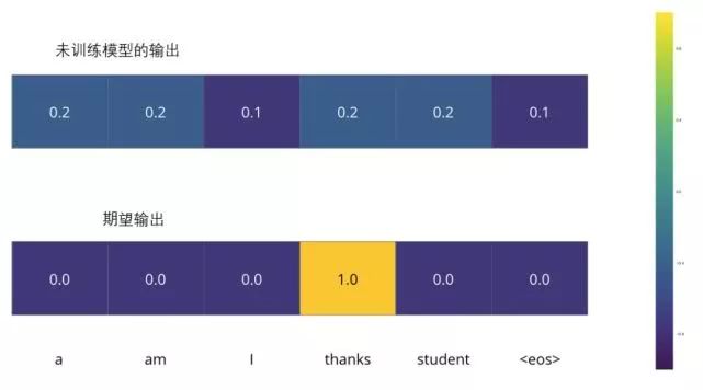
Because the model’s parameters (weights) are generated randomly, the (untrained) model assigns random values to the probability distribution in each cell/word. We can compare it with the actual output and then slightly adjust all model weights using the backpropagation algorithm to generate outputs that are closer to the result.
How would you compare two probability distributions? We can simply subtract one from the other. For more details, refer to cross-entropy and KL divergence.
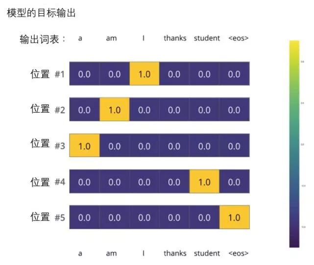
But note that this is a simplified example. A more realistic scenario is handling a sentence. For example, input “je suis étudiant” and expect the output to be “i am a student.” We want our model to successfully output probability distributions in these cases:
Each probability distribution is represented by a vector of the same width as the vocabulary size (in our example, it is 6, but in reality, it is usually 3000 or 10000).
The first probability distribution has the highest probability in the cell associated with “i.”
The second probability distribution has the highest probability in the cell associated with “am.”
And so on, the fifth output distribution indicates the highest probability in the cell associated with “” (the end of sentence).
After sufficiently training on a large dataset, we expect the probability distribution output by the model to look like this: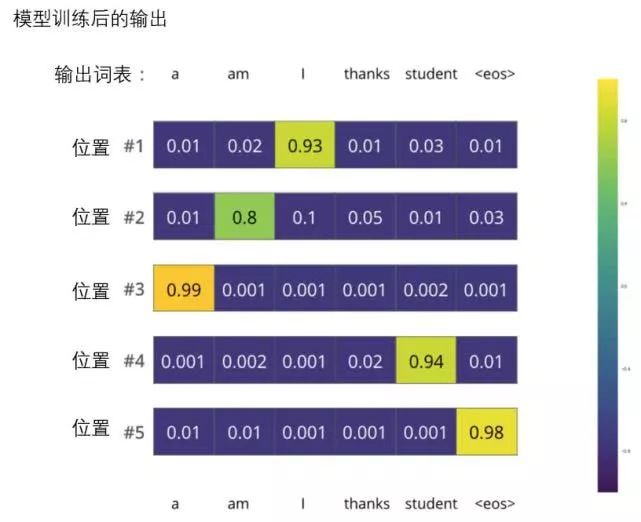
We expect that after training, the model will output the correct translation. Of course, if this sentence comes entirely from the training set, it is not a good evaluation metric. Note that each position (word) receives a bit of probability, even if it is unlikely to be the output at that time step — this is a useful property of softmax that helps the model train.
Since this model produces one output at a time, let’s assume this model only chooses the word with the highest probability and discards the rest. This is one method (called greedy decoding). Another method to accomplish this task is to retain the top two words with the highest probabilities (for example, “I” and “a”), and then run the model twice for the next step: once assuming the first position outputs the word “I,” and another assuming it outputs the word “me,” and whichever version produces less error retains the highest probability translation. Then we repeat this step for the second and third positions. This method is called beam search (in our example, the beam width is 2 because it retains two beam results, such as the first and second positions), and it ultimately returns two beam results (top_beams is also 2). These are all parameters that can be set in advance.
Further Steps
I hope the above has helped you understand the main concepts of the Transformer. If you want to delve deeper into this field, I suggest the following steps: read Attention Is All You Need, the Transformer blog, and the Tensor2Tensor announcement, and check out Łukasz Kaiser’s introduction to understand the model and its details.
Editor: Yu Tengkai
Proofread by: Lin Yilin