Introduction to TensorFlow Feature Columns

Written by / TensorFlow Team

Welcome to the second part of the introduction to TensorFlow Datasets and Estimators series (click here for the first part). In this article, we will introduce Feature Columns – a data structure that describes the features needed for the estimator to train and make predictions. As you will see below, the information in feature columns is very rich, allowing you to represent various types of data.

In Part 1 (Introduction to TensorFlow Datasets and Estimators), we used the pre-built estimator DNNClassifier to train a model to predict different types of Iris flowers based on our input features. That example only created numeric feature columns (of type tf.feature_column.numeric_column). While those feature columns are sufficient to model the lengths of petals and sepals, real-world datasets often contain various non-numeric features. For example:

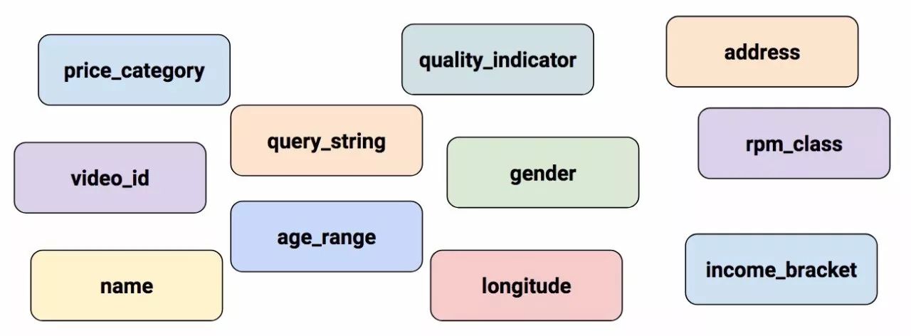
Figure 1. Non-numeric features.

How can we represent non-numeric feature types? That is exactly what we will discuss in this article.

Input to Deep Neural Networks

Let’s start with a question: what kind of data are we actually inputting into deep neural networks? Of course, the answer is numbers (for example, tf.float32). After all, every neuron in a neural network performs multiplication and addition operations on weights and input data. However, real-world input data often contains non-numeric (categorical) data. For example, suppose there is a product_class feature containing the following three non-numeric values:

• kitchenware

• electronics

• sports

Machine learning models typically represent categorical values as simple vectors, where 1 indicates the presence of a value and 0 indicates its absence. For instance, when product_class is set to sports, the machine learning model would typically represent product_class as [0, 0, 1], meaning:

• 0: kitchenware does not exist

• 0: electronics does not exist

• 1: sports exists

Thus, although the original data can be numeric or categorical, machine learning models will represent all features as numbers or vectors composed of numbers.

Introduction to Feature Columns

As shown in Figure 2, you can specify the model’s input through the feature_columns parameter of the estimator (DNNClassifier for Iris). Feature columns connect the input data (returned by input_fn) to your model.

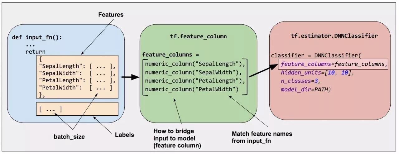
Figure 2. Feature columns link raw data to the data your model needs.

To represent features as feature columns, call functions from the tf.feature_column package. This article will introduce nine functions in this package. As shown in Figure 3, all nine functions return either a Categorical-Column or Dense-Column object, except for bucketized_column, which inherits from both categories:

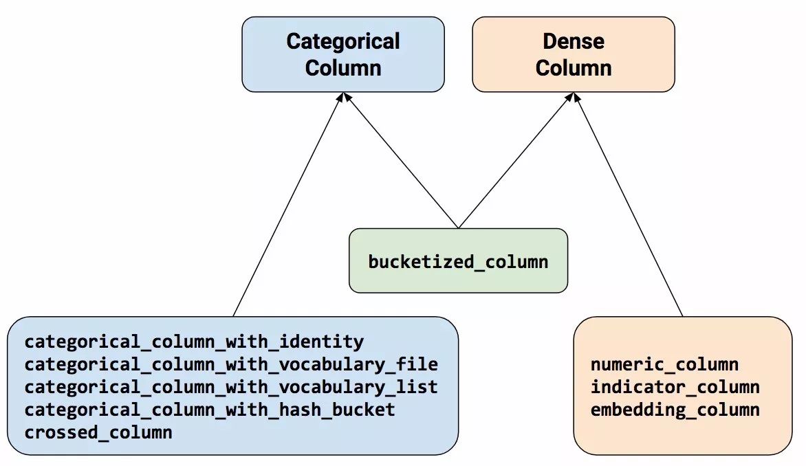
Figure 3. Feature column functions can be categorized into two main categories and one mixed category.

Let’s take a closer look at these functions.

Numeric Column

The Iris classifier calls tf.numeric_column() for all input features: SepalLength, SepalWidth, PetalLength, PetalWidth. Although tf.numeric_column() provides optional parameters, calling the function without any parameters is a very simple way to specify numeric values as model input with a default data type (tf.float32). For example:

# Defaults to a tf.float32 scalar.
numeric_feature_column = tf.feature_column.numeric_column(key="SepalLength")

Using the dtype parameter allows you to specify a non-default numeric data type. For example:

# Represent a tf.float64 scalar.
numeric_feature_column = tf.feature_column.numeric_column(key="SepalLength",
                                                          dtype=tf.float64)

By default, a numeric column can create a single value (scalar). Using the shape parameter allows you to specify another shape. For example:

# Represent a 10-element vector in which each cell contains a tf.float32.
vect_feature_column = tf.feature_column.numeric_column(key="Bowling",
                                                         shape=10)

# Represent a 10x5 matrix in which each cell contains a tf.float32.
matrix_feature_column = tf.feature_column.numeric_column(key="MyMatrix",
                                                         shape=[10,5]) 

Bucketized Column

Generally, you do not want to provide numbers directly to the model; instead, you want to split their values into different categories based on numeric ranges. To do this, create a bucketized column. For example, suppose there is raw data representing the year a house was built. Instead of representing the year as a scalar numeric column, we can split the year into the following four buckets:

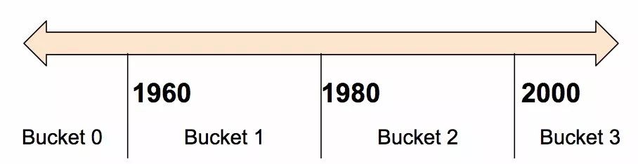
Figure 4. Splitting year data into four buckets.

The model will represent the buckets as follows:

Date Range	Representation…
< 1960	[1, 0, 0, 0]
>= 1960 and < 1980	[0, 1, 0, 0]
>= 1980 and < 2000	[0, 0, 1, 0]
> 2000	[0, 0, 0, 1]

Now, since numbers are a very effective input for the model, why split them into such categorical values? Note that categorization can split an input number into a four-element vector. Thus, the model can learn four separate weights instead of just one. Compared to a single weight, four weights can create a more informative model. More importantly, since only one element is set (1) and the other three are zeroed (0), bucketing allows the model to clearly distinguish between different year categories. If we only used a single number (the year) as input, the model would not be able to distinguish categories. Therefore, bucketing can provide the model with additional important information to learn.

The following code demonstrates how to create a bucketized feature:

# A numeric column for the raw input.
numeric_feature_column = tf.feature_column.numeric_column("Year")

# Bucketize the numeric column on the years 1960, 1980, and 2000
bucketized_feature_column = tf.feature_column.bucketized_column(
    source_column = numeric_feature_column,
    boundaries = [1960, 1980, 2000])

Note the following:

• Before creating the bucketized column, we first created a numeric column to represent the raw year.

• We passed the numeric column as the first parameter to tf.feature_column.bucketized_column().

• Specifying a three-element boundaries vector creates a four-element bucketized vector.

Categorical Identity Column

Categorical identity columns are a special type of bucketized column. In a traditional bucketized column, each bucket represents a range of values (e.g., from 1960 to 1979). In a categorical identity column, each bucket represents a unique integer. For example, suppose you want to represent the integer range [0, 4) (i.e., you want to represent integers 0, 1, 2, or 3). In this case, the categorical identity mapping would look like this:

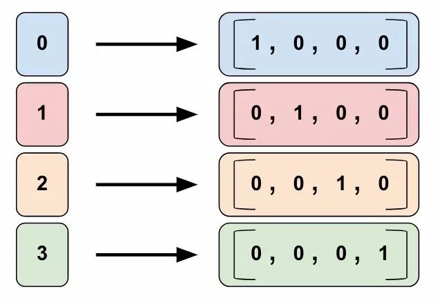
Figure 5. Categorical identity mapping. Note that this is a one-hot encoding, not a binary digit encoding.

So why would you want to represent values with a categorical identity column? Using a bucketized column, the model can learn separate weights for each category in a categorical identity column. For instance, instead of using a string to represent product_class, we use a unique integer value for each category. That is:

• 0=”kitchenware”

• 1=”electronics”

• 2=”sport”

Call tf.feature_column.categorical_column_with_identity() to implement a categorical identity column. For example:

# Create a categorical output for input "feature_name_from_input_fn",
# which must be of integer type. Value is expected to be >= 0 and < num_buckets
identity_feature_column = tf.feature_column.categorical_column_with_identity(
    key='feature_name_from_input_fn', 
    num_buckets=4) # Values [0, 4)

# The 'feature_name_from_input_fn' above needs to match an integer key that is 
# returned from input_fn (see below). So for this case, 'Integer_1' or
# 'Integer_2' would be valid strings instead of 'feature_name_from_input_fn'.
# For more information, please check out Part 1 of this blog series.
def input_fn():
    ...<code>...
    return ({ 'Integer_1':[values], ..<etc>.., 'Integer_2':[values] },
            [Label_values])

Categorical Vocabulary Column

We cannot input strings directly into the model. Instead, we must first map the strings to numbers or categorical values. Categorical vocabulary columns provide a good way to represent strings as one-hot vectors. For example:

Figure 6. Mapping string values to vocabulary columns.

As you can see, categorical vocabulary columns are an enumerated version of categorical identity columns. TensorFlow provides two different functions for creating categorical vocabulary columns:

• tf.feature_column.categorical_column_with_vocabulary_list()

• tf.feature_column.categorical_column_with_vocabulary_file()

The tf.feature_column.categorical_column_with_vocabulary_list() function can map each string to an integer based on an explicit vocabulary list. For example:

# Given input "feature_name_from_input_fn" which is a string,
# create a categorical feature to our model by mapping the input to one of 
# the elements in the vocabulary list.
vocabulary_feature_column =
    tf.feature_column.categorical_column_with_vocabulary_list(
        key="feature_name_from_input_fn",
        vocabulary_list=["kitchenware", "electronics", "sports"]) 

The previous function has a notable drawback; that is, when the vocabulary list is long, a lot of input work is required. For such cases, call tf.feature_column.categorical_column_with_vocabulary_file() instead, which allows you to place the vocabulary in a separate file. For example:

# Given input "feature_name_from_input_fn" which is a string,
# create a categorical feature to our model by mapping the input to one of 
# the elements in the vocabulary file
vocabulary_feature_column =
    tf.feature_column.categorical_column_with_vocabulary_file(
        key="feature_name_from_input_fn",
        vocabulary_file="product_class.txt",
        vocabulary_size=3)

# product_class.txt should have one line for vocabulary element, in our case:
kitchenware
electronics
sports

Using Hash Buckets to Limit Categories

So far, we have only introduced a small number of categories. For example, our product_class example only has 3 categories. However, the number of categories can often be so large that it is impractical to use a separate category for each vocabulary or integer, as this would consume a lot of memory. For such cases, we can reverse the question and ask ourselves, “How many categories am I willing to use for the input?” In fact, the tf.feature_column.categorical_column_with_hash_buckets() function allows you to specify the number of categories. For example, the following code shows how this function computes the hash value of the input and then uses the modulus operator to place it in one of the hash_bucket_size categories:

# Create categorical output for input "feature_name_from_input_fn".
# Category becomes: hash_value("feature_name_from_input_fn") % hash_bucket_size
hashed_feature_column =
    tf.feature_column.categorical_column_with_hash_bucket(
        key = "feature_name_from_input_fn",
        hash_buckets_size = 100) # The number of categories

At this point, you might think, “This is crazy!” After all, we are forcing different input values into a smaller set of categories. This means that two seemingly unrelated inputs will be mapped to the same category, which is the same for the neural network. Figure 7 illustrates this dilemma, showing that both kitchenware and sports have been assigned category (hash bucket) 12:

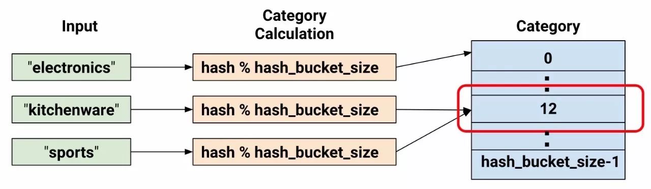
Figure 7. Representing data in hash buckets.

As with many counterintuitive phenomena in machine learning, hashing often works well in practice. This is because hash categories provide some separation for the model. The model can use more features to further separate kitchenware from sports.

Feature Crosses

The last type of categorical column we will introduce allows us to combine multiple input features into one. Combined features (more commonly known as feature crosses) allow the model to learn separate weights specifically for the meaning represented by the combination of features.

To be more specific, suppose we want our model to calculate real estate prices in Atlanta, Georgia. The real estate prices in this city vary greatly depending on location. Representing latitude and longitude as separate features is not very useful in determining the relevance of real estate locations; however, combining latitude and longitude into a single feature can specify location. Suppose we represent Atlanta with a 100×100 rectangular profile grid by crossing latitude and longitude to determine 10,000 profiles. This combination allows the model to pick up pricing conditions related to each profile, providing stronger information compared to latitude and longitude alone.

Figure 8 shows our map, which includes latitude and longitude values for the four corners of the city:

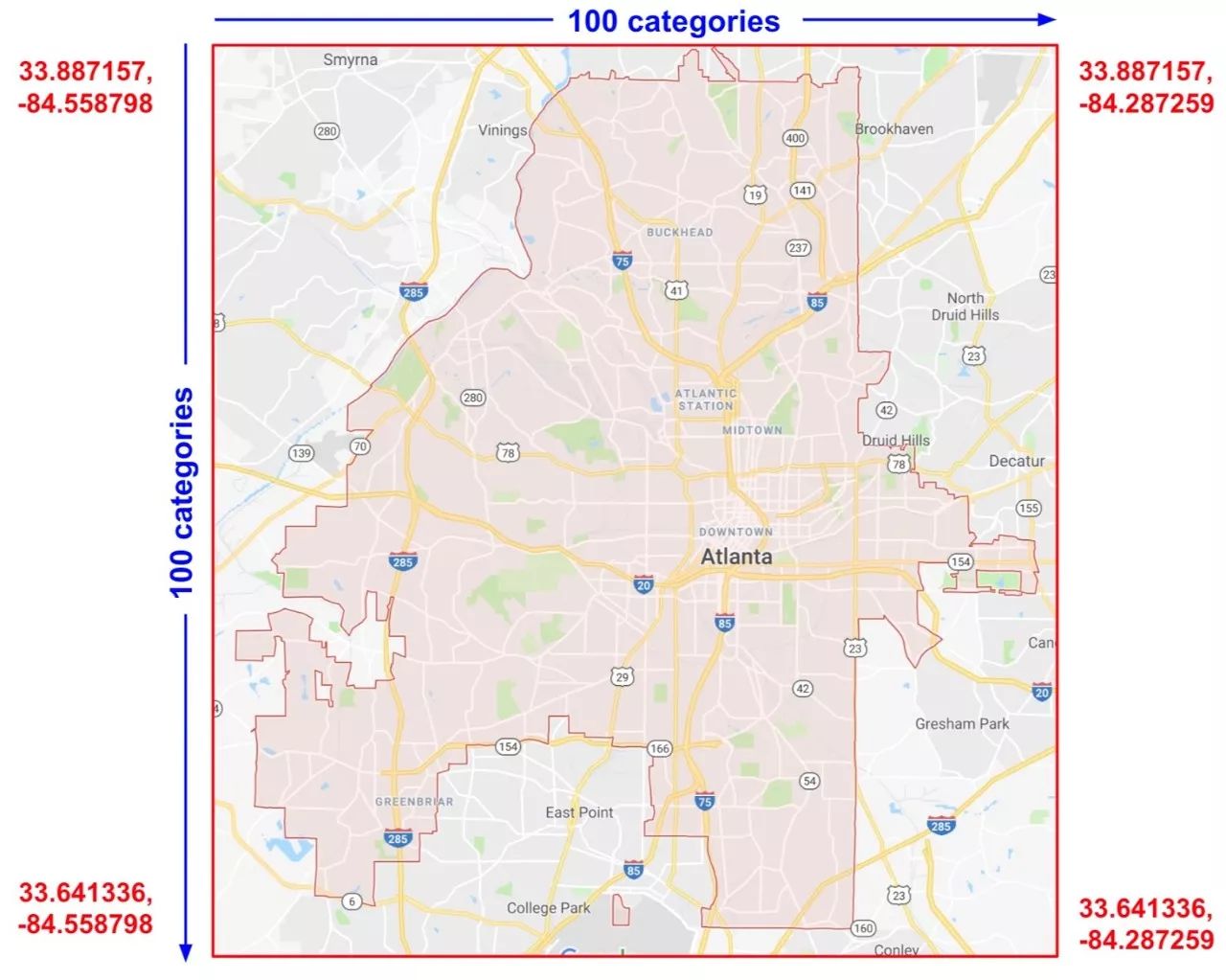
Figure 8. Atlanta map. Imagine this map is made up of 10,000 equal-sized profiles.

To solve the problem, we use some of the previously introduced feature columns and the tf.feature_columns.crossed_column() function.

# In our input_fn, we convert input longitude and latitude to integer values
# in the range [0, 100)
def input_fn():
    # Using Datasets, read the input values for longitude and latitude
    latitude = ...   # A tf.float32 value
    longitude = ...  # A tf.float32 value

    # In our example we just return our lat_int, long_int features.
    # The dictionary of a complete program would probably have more keys.
    return { "latitude": latitude, "longitude": longitude, ...}, labels

# As can be see from the map, we want to split the latitude range
# [33.641336, 33.887157] into 100 buckets. To do this we use np.linspace
# to get a list of 99 numbers between min and max of this range.
# Using this list we can bucketize latitude into 100 buckets.
latitude_buckets = list(np.linspace(33.641336, 33.887157, 99))
latitude_fc = tf.feature_column.bucketized_column(
    tf.feature_column.numeric_column('latitude'),
    latitude_buckets)

# Do the same bucketization for longitude as done for latitude.
longitude_buckets = list(np.linspace(-84.558798, -84.287259, 99))
longitude_fc = tf.feature_column.bucketized_column(
    tf.feature_column.numeric_column('longitude'), longitude_buckets)

# Create a feature cross of fc_longitude x fc_latitude.
fc_san_francisco_boxed = tf.feature_column.crossed_column(
    keys=[latitude_fc, longitude_fc],
    hash_bucket_size=1000) # No precise rule, maybe 1000 buckets will be good?

You can create feature crosses from one of the following:

• Feature names; that is, names from the dict returned from input_fn.

• Any categorical column (see Figure 3), except for categorical_column_with_hash_bucket.

When the feature columns latitude_fc and longitude_fc are crossed, TensorFlow will create 10,000 combinations of (latitude_fc, longitude_fc) organized as follows:

(0,0),(0,1)...  (0,99)
(1,0),(1,1)...  (1,99)
…, …,          ...
(99,0),(99,1)...(99, 99)

The tf.feature_column.crossed_column function will perform hash calculations on these combinations and insert the results into categories using the hash_bucket_size, as discussed earlier. As with previous discussions, performing hash and modulus functions will likely result in category collisions; that is, multiple (latitude, longitude) feature crosses will appear in the same hash bucket. However, in practice, performing feature crosses can still provide valuable insights for the model’s learning capability.

Somewhat counterintuitively, when creating feature crosses, you typically still need to include the original (non-crossed) features in the model. For example, you need to provide both (latitude, longitude) feature crosses and the latitude and longitude as separate features. The separate latitude and longitude features will help the model separate the contents of hash buckets containing different feature crosses.

For a complete code example, see this link:

https://github.com/tensorflow/models/blob/master/samples/outreach/blogs/housing_prices.ipynb

Additionally, the “Resources” section at the end of this article provides more examples of feature crosses.

Indicator and Embedding Columns

Indicator and embedding columns never operate directly on features but take categorical columns as input.

When using indicator columns, we will inform TensorFlow to accurately perform the operation we saw in the categorical product_class example. That is, indicator columns treat each category as an element in a one-hot vector, where the matching category’s value is 1, and the rest are 0:

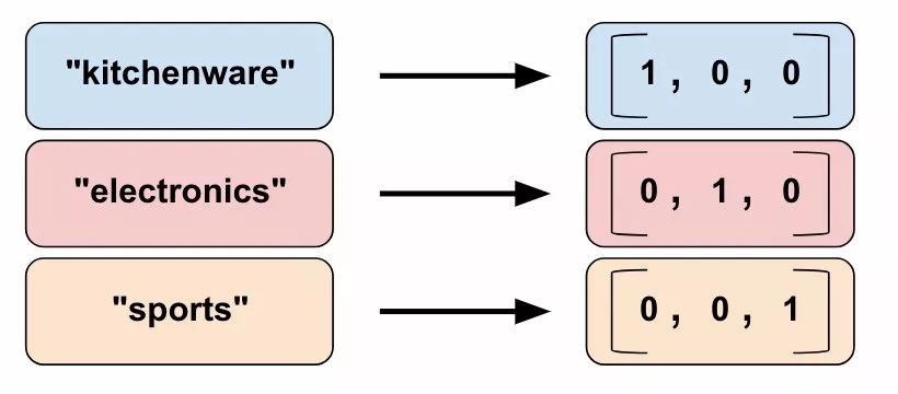
Figure 9. Representing data in indicator columns.

Here is how to create an indicator column:

categorical_column = ... # Create any type of categorical column, see Figure 3

# Represent the categorical column as an indicator column.
# This means creating a one-hot vector with one element for each category.
indicator_column = tf.feature_column.indicator_column(categorical_column)

Now, suppose we have not just three possible categories, but one million. Or one billion. For various reasons (too technical to cover here), training a neural network with a large number of categories using indicator columns will become impractical.

We can overcome this limitation by using embedding columns. Instead of representing data as a one-hot vector with many dimensions, embedding columns represent data as a regular vector of lower dimensions, where each cell can contain any number, not just 0 or 1. By allowing richer numerical combinations in each cell, embedding columns can contain far fewer cells than indicator columns.

Let’s look at an example comparing indicator columns and embedding columns. Suppose our input examples contain different words from a finite combination that only has 81 words. Now suppose the dataset provides the following input words in four separate examples:

• “dog”

• “spoon”

• “scissors”

• “guitar”

In this case, Figure 10 illustrates the processing paths for embedding columns or indicator columns.

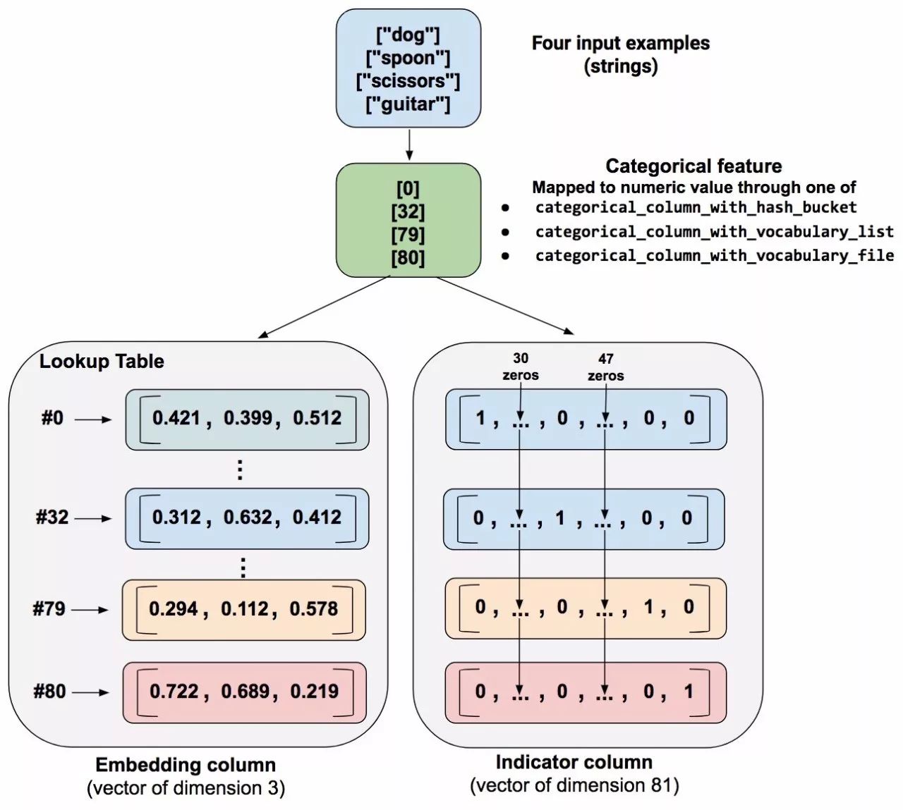
Figure 10. Compared to indicator columns, embedding columns store categorical data in a lower-dimensional vector. (We are just placing random numbers in the embedding vector; training determines the actual numbers.)

When processing an example, a categorical_column_with… function maps the example string to numeric categorical values. For example, a function might map “spoon” to [32]. (32 comes from our imagination – actual values depend on the mapping function.) You can then represent these numeric categorical values in one of two ways:

• As an indicator column. The function converts each numeric categorical value into an 81-element vector (since our combination contains 81 words), placing 1 at the indices of the categorical values (0, 32, 79, 80) and 0 elsewhere.

• As an embedding column. A function uses the numeric categorical values (0, 32, 79, 80) as indices for a lookup table. Each display position in the lookup table contains a 3-element vector.

How are the values in the embedding vector magically assigned? In fact, the assignment occurs during training. That is, the model will learn the best way to map your input numeric categorical values to embedding vector values, solving your problem. Embedding columns can enhance your model’s capabilities because embedding vectors can learn new relationships between categories from training data.

Why is the size of the vector in our example 3? The following “formula” provides a general rule of thumb related to the number of embedding dimensions:

embedding_dimensions =  number_of_categories**0.25

That is, the number of embedding vector dimensions should be the fourth root of the number of categories. Since the vocabulary size in this example is 81, the suggested number of dimensions is 3:

3 =  81**0.25

Note that this is just a general guideline; you can set the number of embedding dimensions as you wish.

Call tf.feature_column.embedding_column to create an embedding_column. The dimensions of the embedding vector depend on the problem at hand, but common values can start from as low as 3 up to 300 or more:

categorical_column = … # Create any categorical column shown in Figure 3.

categorical_column = ... # Create any categorical column shown in Figure 3.

# Represent the categorical column as an embedding column.
# This means creating a one-hot vector with one element for each category.
embedding_column = tf.feature_column.embedding_column(
    categorical_column=categorical_column,
    dimension=dimension_of_embedding_vector)

Embedding is a big topic in machine learning. This information aims to help you get started using them as feature columns. Please see the resources at the end of this article for more information.

Passing Feature Columns to Estimators

Still with us? I hope everyone is still following along because the fundamentals of feature columns are about to be wrapped up.

As we saw in Figure 1, feature columns can map your input data (described through the feature dictionary returned from input_fn) to the values you provide to the model. Specify feature columns to the estimator’s feature_columns parameter as a list. Note that the feature_columns parameter varies depending on the estimator:

LinearClassifier and LinearRegressor:

• Accept all types of feature columns.

DNNClassifier and DNNRegressor:

• Only accept dense columns, see Figure 3. As mentioned earlier, other column types must be wrapped in indicator_column or embedding_column.

DNNLinearCombinedClassifier and DNNLinearCombinedRegressor:

• linear_feature_columns parameter can accept any column type, just like the above LinearClassifier and LinearRegressor.

• However, the dnn_feature_columns parameter is limited to dense columns, like the above DNNClassifier and DNNRegressor.

The reasons for the above rules go beyond the scope of this introductory article, but we will ensure to cover this in future articles.

Conclusion

Using feature columns allows you to map your input data to the representations you provide to the model. In Part 1 of this series, we only used numeric_column, but with the other functions introduced in this article, you can easily create additional feature columns.

For more detailed information about feature columns, please refer to the resources below:

• Video by Josh Gordon introducing feature engineering

• Jupyter notebook from the same author

• TensorFlow – Wide & Deep tutorial

• Examples of DNN and linear models using feature columns

If you want to learn more about embeddings, please refer to the following resources:

• Deep Learning, NLP, and Representation (Colah’s blog)

• Refer to TensorFlow Embedding Projector

How to refer? Please reply to this public account with “Feature Column Resources” to get resource links.