Written by / Li Xihan, Google Developers Expert
This article is excerpted from “Simple and Rough TensorFlow 2.0”
In the previous article, we introduced the widely used convolutional neural networks in the field of images and their implementation in TensorFlow 2.0. This article continues to introduce another widely popular neural network architecture, namely the recurrent neural network, with the following content:
- Using text auto-generation tasks as an example, we will introduce the implementation of recurrent neural networks in TensorFlow 2.0;
-
Introduce the principles of recurrent neural networks for beginners in deep learning.
Building a text generation model based on recurrent neural networks using Keras
Recurrent Neural Networks (RNN) are a type of neural network suitable for processing sequential data and are widely used in language models, text generation, machine translation, etc.
Basic Knowledge and Principles
Recurrent Neural Networks Tutorial, Part 1 – Introduction to RNNs
Professor Li Hongyi from National Taiwan University’s course on Recurrent Neural Network (part 1) and Recurrent Neural Network (part 2).
LSTM Principles: Understanding LSTM Networks
Graves, Alex. “Generating Sequences With Recurrent Neural Networks.” ArXiv:1308.0850 [Cs], August 4, 2013. (http://arxiv.org/abs/1308.0850).
Here, we use RNN to automatically generate text in the style of Nietzsche. [5]
This task essentially predicts the probability distribution of the next letter in a segment of English text. For example, we have the following sentence: I am a studen. This sentence (sequence) contains 13 characters (including spaces). When we read this sequence of 13 characters, based on our experience, we can predict that the next character is most likely “t”. We hope to build a model that takes a sequence of length seq_length as input and outputs the probability distribution of the next character in these sequences. We sample from the probability distribution of the next character as the predicted value, then we can generate the next two characters, three characters, etc., completing the text generation task. First, we will implement a simple DataLoader class to read the text and encode it character by character. Let the number of character types be num_chars, assigning a unique integer index i between 0 and num_chars - 1 to each character.
1class DataLoader():
2    def __init__(self):
3        path = tf.keras.utils.get_file('nietzsche.txt',
4            origin='https://s3.amazonaws.com/text-datasets/nietzsche.txt')
5        with open(path, encoding='utf-8') as f:
6            self.raw_text = f.read().lower()
7        self.chars = sorted(list(set(self.raw_text)))
8        self.char_indices = dict((c, i) for i, c in enumerate(self.chars))
9        self.indices_char = dict((i, c) for i, c in enumerate(self.chars))
10        self.text = [self.char_indices[c] for c in self.raw_text]
11
12    def get_batch(self, seq_length, batch_size):
13        seq = []
14        next_char = []
15        for i in range(batch_size):
16            index = np.random.randint(0, len(self.text) - seq_length)
17            seq.append(self.text[index:index+seq_length])
18            next_char.append(self.text[index+seq_length])
19        return np.array(seq), np.array(next_char)       # [batch_size, seq_length], [num_batch]
Next, we will implement the model. In the __init__ method, we instantiate a commonly used LSTMCell unit and a fully connected layer for linear transformation. We first perform a “One Hot” operation on the sequence, converting the encoding i of each character in the sequence into a num_char dimensional vector, where the i-th position is 1 and the others are 0. The shape of the transformed sequence tensor is [seq_length, num_chars]. Then, we initialize the state of the RNN unit and store it in a variable state. Next, we sequentially feed the sequence into the RNN unit from start to end. At time t, we feed the previous time step t-1’s RNN unit state state and the t-th element of the sequence inputs[t, :] into the RNN unit to obtain the current output output and the RNN unit state. We take the last output of the RNN unit and transform it through the fully connected layer to a num_chars dimensional vector, which serves as the model’s output.

output, state = self.cell(inputs[:, t, :], state) Diagram
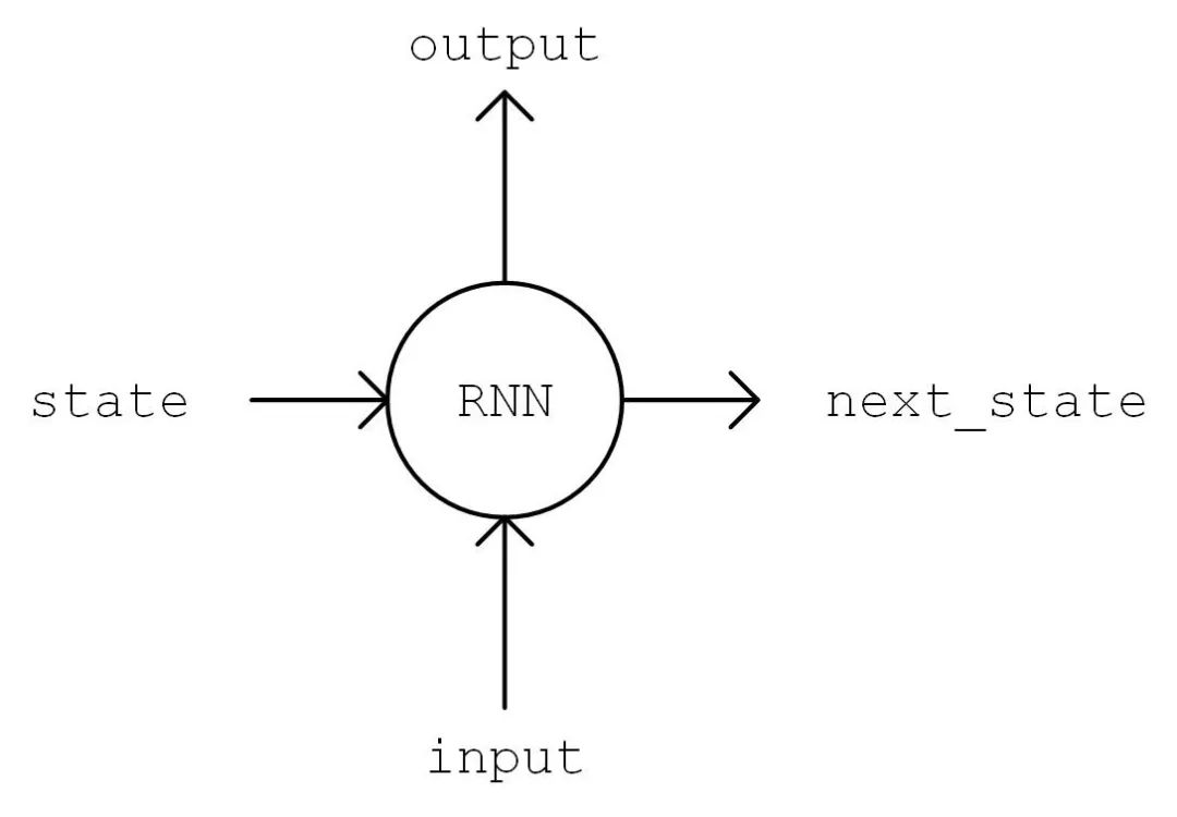
RNN Process Flow Diagram
The specific implementation is as follows:
1class RNN(tf.keras.Model):
2    def __init__(self, num_chars, batch_size, seq_length):
3        super().__init__()
4        self.num_chars = num_chars
5        self.seq_length = seq_length
6        self.batch_size = batch_size
7        self.cell = tf.keras.layers.LSTMCell(units=256)
8        self.dense = tf.keras.layers.Dense(units=self.num_chars)
9
10    def call(self, inputs, from_logits=False):
11        inputs = tf.one_hot(inputs, depth=self.num_chars)       # [batch_size, seq_length, num_chars]
12        state = self.cell.get_initial_state(batch_size=self.batch_size, dtype=tf.float32)
13        for t in range(self.seq_length):
14            output, state = self.cell(inputs[:, t, :], state)
15        logits = self.dense(output)
16        if from_logits:
17            return logits
18        else:
19            return tf.nn.softmax(logits)
Define some model hyperparameters:
1    num_batches = 1000
2    seq_length = 40
3    batch_size = 50
4    learning_rate = 1e-3
The training process is basically consistent with the previous articles in this series, summarized as follows:
- Randomly sample a batch of training data from
DataLoader; -
Feed this batch of data into the model and compute the model’s predictions;
-
Compare the model’s predictions with the true values and compute the loss function;
-
Compute the gradient of the loss function with respect to the model variables;
- Use the optimizer to update the model parameters to minimize the loss function.
1    data_loader = DataLoader()
2    model = RNN(num_chars=len(data_loader.chars), batch_size=batch_size, seq_length=seq_length)
3    optimizer = tf.keras.optimizers.Adam(learning_rate=learning_rate)
4    for batch_index in range(num_batches):
5        X, y = data_loader.get_batch(seq_length, batch_size)
6        with tf.GradientTape() as tape:
7            y_pred = model(X)
8            loss = tf.keras.losses.sparse_categorical_crossentropy(y_true=y, y_pred=y_pred)
9            loss = tf.reduce_mean(loss)
10            print("batch %d: loss %f" % (batch_index, loss.numpy()))
11        grads = tape.gradient(loss, model.variables)
12        optimizer.apply_gradients(grads_and_vars=zip(grads, model.variables))
There is one point that needs special attention regarding the text generation process. Previously, we always used the tf.argmax() function to take the value with the highest probability as the prediction. However, for text generation, this prediction method is too absolute and can cause the generated text to lose richness. Therefore, we use the np.random.choice() function to sample according to the generated probability distribution. This way, even characters with relatively low probabilities have a chance to be sampled. At the same time, we introduce a temperature parameter to control the shape of the distribution; a larger parameter value makes the distribution flatter (the difference between the maximum and minimum values is smaller), increasing the richness of the generated text, while a smaller parameter value makes the distribution steeper, decreasing the richness of the generated text.
1    def predict(self, inputs, temperature=1.):
2        batch_size, _ = tf.shape(inputs)
3        logits = self(inputs, from_logits=True)
4        prob = tf.nn.softmax(logits / temperature).numpy()
5        return np.array([np.random.choice(self.num_chars, p=prob[i, :])
6                         for i in range(batch_size.numpy())])
By using this method for continuous prediction in a “snowball” manner, we can obtain the generated text.
1    X_, _ = data_loader.get_batch(seq_length, 1)
2    for diversity in [0.2, 0.5, 1.0, 1.2]:
3        X = X_
4        print("diversity %f:" % diversity)
5        for t in range(400):
6            y_pred = model.predict(X, diversity)
7            print(data_loader.indices_char[y_pred[0]], end='', flush=True)
8            X = np.concatenate([X[:, 1:], np.expand_dims(y_pred, axis=1)], axis=-1)
9        print("\n")
The generated text is as follows:
 1diversity 0.200000:
 2conserted and conseive to the conterned to it is a self--and seast and the selfes as a seast the expecience and and and the self--and the sered is a the enderself and the sersed and as a the concertion of the series of the self in the self--and the serse and and the seried enes and seast and the sense and the eadure to the self and the present and as a to the self--and the seligious and the enders
 3
 4diversity 0.500000:
 5can is reast to as a seligut and the complesed
 6has fool which the self as it is a the beasing and us immery and seese for entoured underself of the seless and the sired a mears and everyther to out every sone thes and reapres and seralise as a streed liees of the serse to pease the cersess of the selung the elie one of the were as we and man one were perser has persines and conceity of all self-el
 7
 8diversity 1.000000:
 9entoles by
10their lisevers de weltaale, arh pesylmered, and so jejurted count have foursies as is
11descinty iamo; to semplization refold, we dancey or theicks-welf--atolitious on his
12such which
13here
14oth idey of pire master, ie gerw their endwit in ids, is an trees constenved mase commars is leed mad decemshime to the mor the elige. the fedies (byun their ope wopperfitious--antile and the it as the f
15
16diversity 1.200000:
17cain, elvotidue, madehoublesily
18inselfy!--ie the rads incults of to prusely le]enfes patuateded:.--a coud--theiritibaior "nrallysengleswout peessparify oonsgoscess teemind thenry ansken suprerial mus, cigitioum: 4reas. whouph: who
19eved
20arn inneves to sya" natorne. hag open reals whicame oderedte,[fingo is
21zisternethta simalfule dereeg hesls lang-lyes thas quiin turjentimy; periaspedey tomm--whach
[5] This task and implementation refer to:
The Working Process of Recurrent Neural Networks Recurrent Neural Networks are a neural network structure that processes time series data, meaning we need to have a timeline in our minds. The recurrent neural network has an initial state
. At each time point
it iteratively processes the current time input
, modifies its own state
, and produces output
. The core of the recurrent neural network is the state
, which is a vector of a specific dimension, similar to the “memory” of a neural network. At the initial moment
we assume
has been computed, focusing on how to compute
:
Linearly transform the input vector
through the matrix
, which has the same dimension as state s;
Linearly transform
through the matrix
, which has the same dimension as state s;
Add the two vectors obtained above and apply an activation function to obtain the value of the current state
, that is,
. In other words, the value of the current state is generated by integrating the value of the previous state and the current input;
Linearly transform the current state
through the matrix
, to obtain the output at the current time
.
RNN Working Process Diagram (from http://www.wildml.com/2015/09/recurrent-neural-networks-tutorial-part-1-introduction-to-rnns/)
We assume that the dimensions of the input vector
, state
, and output vector
are
,
,
respectively, then
,
,
.
In practice, some common improvements such as LSTM (Long Short-Term Memory networks, which solve the gradient vanishing problem for long sequences and are suitable for longer sequences) and GRU are often used.
Benefits | Q&A Session
We know that there are many challenges and difficulties to overcome when starting a new technology. If you have any questions related to TensorFlow, please leave a comment at the end of this article, and our engineers and GDE will select some representative questions to answer in the next issue~
In the previous article “TensorFlow 2.0 Model: Convolutional Neural Networks”, we answered some representative questions as follows:
Q1:Can you talk about the types of model saving? Previously, TensorFlow 1.x saved as ckpt and then converted to pb. How will TensorFlow 2 save and use it?A: In TensorFlow 2.0, we mainly use tf.train.Checkpoint to save model parameters. Use SavedModel to export the complete model. Please refer to:
Q2:Can the sample code in the article be open-sourced?
A:The original text of this manual is open-sourced on GitHub(https://github.com/snowkylin/tensorflow-handbook), and the sample code can be accessed at (https://github.com/snowkylin/tensorflow-handbook/tree/master/source/_static/code/zh).
Q3:Is there a discussion on distributed systems? It seems that tf’s distributed system is difficult to use.A: TensorFlow 2.0 provides a very user-friendly distributed API tf.distributed, just instantiate a MirroredStrategy strategy:
1strategy = tf.distribute.MirroredStrategy()
And place the model building code within the context of strategy.scope():
1with strategy.scope():
2# Model building code
For multi-machine training, just change MirroredStrategy to MultiWorkerMirroredStrategy. Yes, it’s that simple! We will introduce TensorFlow 2.0’s distributed computing in detail in later installments. More detailed usage methods and examples can be found at:https://tf.wiki/zh/appendix/distributed.htmlQ4: For beginners in TensorFlow, is there a good learning path?A: This series of tutorials “Simple and Rough TensorFlow 2.0” (https://tf.wiki) aims to provide easy-to-follow systematic guidance for TensorFlow beginners. In addition, the official TensorFlow tutorial has been extensively updated to improve readability, which can be referenced at:https://tensorflow.google.cn/overview
Table of Contents for “Simple and Rough TensorFlow 2.0”
-
TensorFlow 2.0 Installation Guide
-
TensorFlow 2.0 Basics: Tensors, Automatic Differentiation, and Optimizers
-
TensorFlow 2.0 Models: Building Model Classes
-
TensorFlow 2.0 Models: Multi-Layer Perceptrons
-
TensorFlow 2.0 Models: Convolutional Neural Networks
-
TensorFlow 2.0 Models: Recurrent Neural Networks (This Article)
Reply with the keyword “Manual” to obtain a collection of series content and FAQs.