Understanding Transformer Principles and Implementation in 10 Minutes

Follow the public account “ML_NLP“

Set as “Starred“, heavy content delivered first-hand!

Source | Zhihu

Address | https://zhuanlan.zhihu.com/p/80986272

Author | Chen Chen

Editor | Machine Learning Algorithms and Natural Language Processing Public Account

This article is for academic sharing only. If there is any infringement, please contact us to delete the article.

The model built on the Transformer, as described in “Attention Is All You Need” (such as BERT), has achieved revolutionary results in multiple natural language processing tasks, and has now replaced RNN as the default option, showcasing the power of Transformer.

Combining Harvard’s code “Annotated Transformer”, let’s share this encoder-decoder method combined with the attention mechanism. Code link: The Annotated Transformer.

Table of Contents:

1. Overall Architecture Description

2. Input & Output Embedding

1. OneHot Encoding

2. Word Embedding

3. Positional Embedding

4. Input short summary

3. Encoder

1. Encoder Sub-layer 1: Multi-Head Attention Mechanism

1. Step 1

2. Step 2

3. Step 3

2. Encoder Sub-layer 2: Position-Wise fully connected feed-forward

3. Encoder short summary

4. Decoder

1. Diff_1: “masked” Multi-Headed Attention

2. Diff_2: encoder-decoder multi-head attention

3. Diff_3: Linear and Softmax to Produce Output Probabilities

1. greedy search

2. beam search

3. Scheduled Sampling

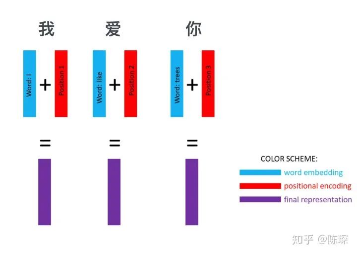
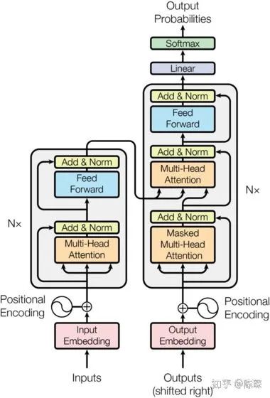
0. Model Architecture:

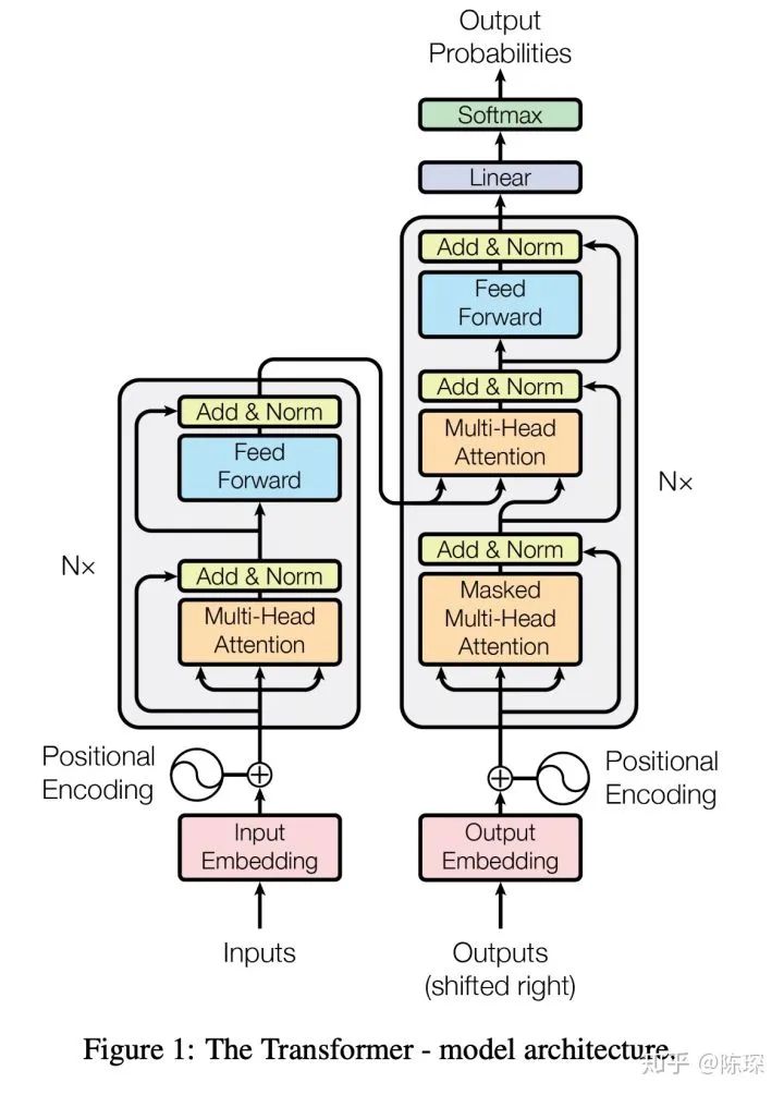
Today’s example task is Chinese to English translation: the Chinese input “我爱你” translates to “I Love You” through the Transformer.

The corresponding hyperparameters in the Transformer include:

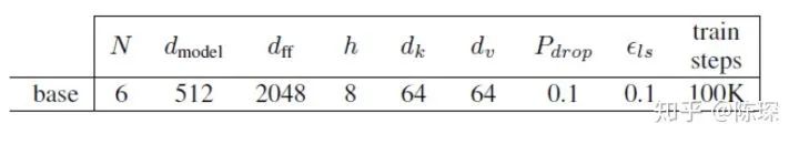
These are also the hyperparameters used in the function make_model(src_vocal, tgt_vocab, N=6, d_model=512, d_ff = 2048, h=8, dropout=0.1).

At first glance, the entire architecture can be quite intimidating, so we need to break down the Transformer into parts:

• Embedding part

• Encoder part

• Decoder part

1. Representing Input and Output

1.1 Representing Input

First, we use the common method for expressing categorical features, which is one-hot encoding, to represent the sentence. One-hot means that a vector has only one element equal to 1, while the others are 0. It’s straightforward; the length of the vector is determined by the length of the vocabulary. If we want to express 10,000 words, we need a 10,000-dimensional vector.

1.2 Word Embedding

However, we do not directly input simple one-hot vectors into the Transformer. The reasons include that this representation is very sparse, very large, and cannot express the features between words. Therefore, we embed words using shorter vectors to represent the attributes of the words. Generally, in PyTorch, we use nn.Embedding to do this, or we can directly multiply the one-hot vector with a weight matrix W.

nn.Embedding contains a weight matrix W, with the shape (num_embeddings, embedding_dim). num_embeddings refers to the vocabulary size, that is, the length of the vocabulary we want to translate. embedding_dim refers to how long a vector we want to use to express a word, which can be arbitrarily chosen, such as 64, 128, 256, 512, etc. In the Transformer paper, the choice is 512 (i.e., d_model = 512).

In fact, we can visualize nn.Embedding as a lookup table, where each word has a stored vector. For any given word, we can look up the corresponding result from the table.

There are two options for handling the nn.Embedding weight matrix:

• Use pre-trained embeddings and fix them; in this case, it is essentially a lookup table.

• Randomly initialize it (of course, we can also choose pre-trained results), but set it to be trainable. This way, the embeddings are continuously improved during the training process.

The Transformer chooses the latter.

In the Annotated Transformer, the class “Embeddings” is used to generate word embeddings, utilizing nn.Embedding. The specific implementation is as follows:

class Embeddings(nn.Module):
    def __init__(self, d_model, vocab):
        super(Embeddings, self).__init__()
        self.lut = nn.Embedding(vocab, d_model)
        self.d_model = d_model

    def forward(self, x):
        return self.lut(x) * math.sqrt(self.d_model)

1.3 Positional Embedding

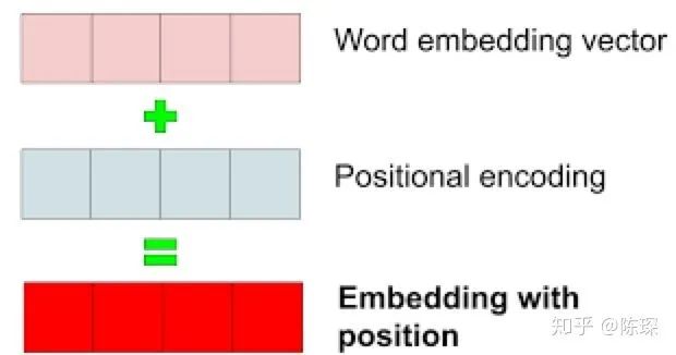
We embed each word to represent input. However, there is still a problem: the embeddings themselves do not contain relative positional information in the sentence.

So why can RNN use the same vector for the same word in any place? Because RNN processes the sentence sequentially, one word at a time. However, in the Transformer, all words in the input sentence are processed simultaneously, without considering the order and positional information of the words.

To solve this problem, the authors of the Transformer proposed the method of adding “positional encoding”. “Positional encoding” allows the Transformer to measure information related to word positions.

Adding positional encoding to word embeddings gives us embeddings with position.

So how exactly is “positional encoding” done? How can it express positional information? The authors explored two methods for creating positional encoding:

• Learn positional encoding vectors through training

• Use a formula to compute positional encoding vectors

After experimentation, it was found that the results of both choices were similar, so the second method was adopted. The advantage is that it does not require training parameters and can be used even for sentence lengths not seen in the training set.

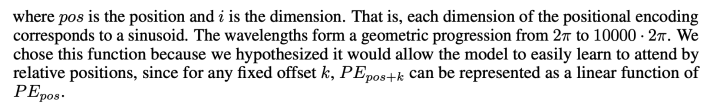
The formula for calculating positional encoding is:

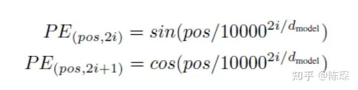
In this formula:

• pos refers to the position of this word in the sentence

• i refers to the embedding dimension. For example, if d_model=512, then i goes from 1 to 512

Why choose sin and cos? Each dimension of positional encoding corresponds to a sine wave. The authors assume this allows the model to learn relatively easily through corresponding positions.

In the Annotated Transformer, the class “Positional Encoding” is used to create positional encoding and add it to the word embedding:

class PositionalEncoding(nn.Module):
    "Implement the PE function."
    def __init__(self, d_model, dropout, max_len=5000):
        super(PositionalEncoding, self).__init__()
        self.dropout = nn.Dropout(p=dropout)

        # Compute the positional encodings once in log space.
        pe = torch.zeros(max_len, d_model)
        position = torch.arange(0, max_len).unsqueeze(1)
        div_term = torch.exp(torch.arange(0, d_model, 2) *
                             -(math.log(10000.0) / d_model))
        pe[:, 0::2] = torch.sin(position * div_term)
        pe[:, 1::2] = torch.cos(position * div_term)
        pe = pe.unsqueeze(0)
        self.register_buffer('pe', pe)

    def forward(self, x):
        x = x + Variable(self.pe[:, :x.size(1)],requires_grad=False)
        return self.dropout(x)

The frequency and offset of the waves are different for each dimension:

1.4 Input Short Summary

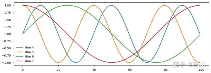
After word embedding and positional embedding, we can obtain a representation of a sentence. For example, the sentence “我爱你” is converted into three vectors, each containing the features of the word and the positional information of the word in the sentence:

We perform the same operation on the output result, which is the English translation “I Love You”. We use word embedding and positional encoding to represent it.

The size of the Input Tensor is [nbatches, L, 512]:

• nbatches refers to the defined batch_size

• L refers to the length of the sequence (for example, “我爱你”, L = 3)

• 512 refers to the embedding dimension

We have now completed the foundational parts of the model architecture:

2. Encoder

The Encoder is slightly more complicated than the Decoder. The Encoder consists of 6 layers stacked together (6 is not fixed and can be modified based on actual conditions), looking like this:

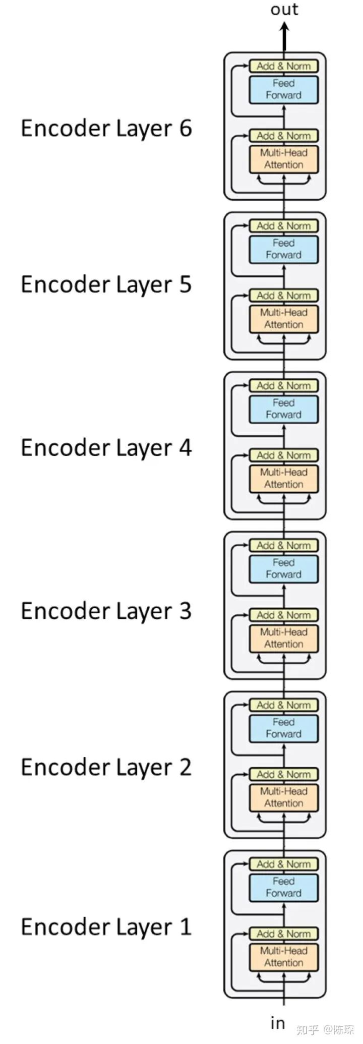
Each layer contains 2 sub-layers:

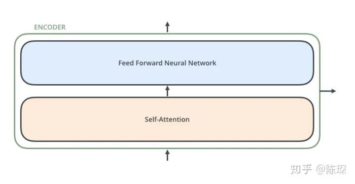
• The first is the “multi-head self-attention mechanism”

• The second is the “simple, position-wise fully connected feed-forward network”

The implementation code of the Encoder in the Annotated Transformer is:

class Encoder(nn.Module):
    "Core encoder is a stack of N layers"

    def __init__(self, layer, N):
        super(Encoder, self).__init__()
        self.layers = clones(layer, N)
        self.norm = LayerNorm(layer.size)

    def forward(self, x, mask):
        "Pass the input (and mask) through each layer in turn."
        for layer in self.layers:
            x = layer(x, mask)
        return self.norm(x)

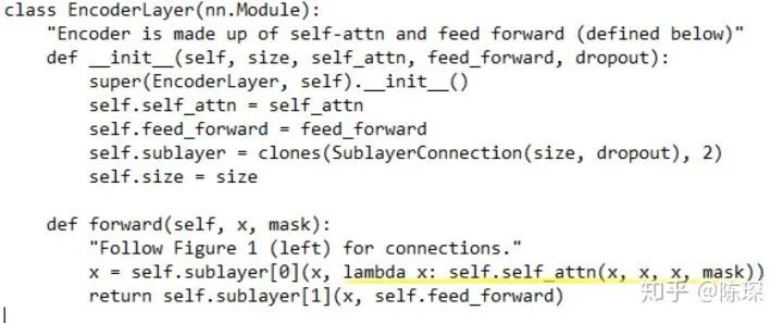
class EncoderLayer(nn.Module):
    "Encoder is made up of self-attn and feed forward (defined below)"
    def __init__(self, size, self_attn, feed_forward, dropout):
        super(EncoderLayer, self).__init__()
        self.self_attn = self_attn
        self.feed_forward = feed_forward
        self.sublayer = clones(SublayerConnection(size, dropout), 2)
        self.size = size

    def forward(self, x, mask):
        "Follow Figure 1 (left) for connections."
        x = self.sublayer[0](x, lambda x: self.self_attn(x, x, x, mask))
        return self.sublayer[1](x, self.feed_forward)

1. The class “Encoder” stacks N times. It is an instance of the class “EncoderLayer”.

2. “EncoderLayer” initialization requires specifying , , , and :

1. corresponds to d_model, which is 512 in the paper

2. is an instance of the class MultiHeadedAttention, corresponding to sub-layer 1

3. is an instance of the class PositionwiseFeedForward, corresponding to sub-layer 2

4. corresponds to the dropout rate

2.1 Encoder Sub-layer 1: Multi-Head Attention Mechanism

Understanding the Multi-Head Attention mechanism is particularly important for understanding the Transformer, and it is used in both the Encoder and Decoder.

Overview: We define the input to the attention mechanism as x. The meaning of x varies at different positions in the Encoder. At the beginning of the Encoder, x represents the representation of the sentence. In the intermediate layers of the EncoderLayer, x represents the output of the previous layer EncoderLayer.

Using different linear layers based on x to calculate keys, queries, and values:

• key = linear_k(x)

• query = linear_q(x)

• value = linear_v(x)

linear_k, linear_q, linear_v are independent and have different weights.

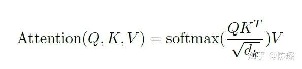
After calculating keys (K), queries (Q), and values (V), the Attention is calculated as follows:

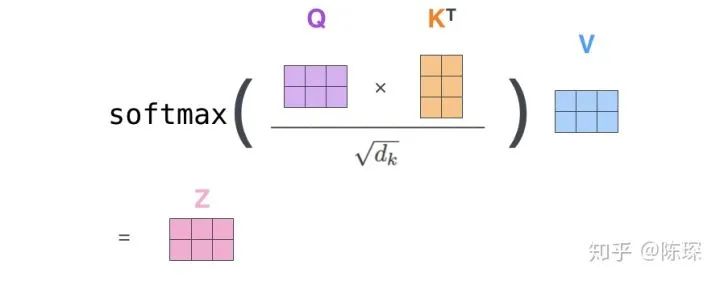
Matrix multiplication representation:

The strange thing here is why we need to divide by sqrt(d_k), right?

The author’s explanation is to prevent the dot product from becoming too large, so we scale it. The original text says, “We suspect that for large values of dk, the dot products grow large in magnitude, pushing the softmax function into regions where it has extremely small gradients”. After applying softmax, the values are all between 0 and 1, and we can understand this as obtaining attention weights. Then, based on these attention weights, we compute the weighted sum of V to get Attention(Q, K, V).

Detailed explanation: The implementation of Multi-Headed attention in the Annotated Transformer is:

class MultiHeadedAttention(nn.Module):
    def __init__(self, h, d_model, dropout=0.1):
        "Take in model size and number of heads."
        super(MultiHeadedAttention, self).__init__()
        assert d_model % h == 0
        # We assume d_v always equals d_k
        self.d_k = d_model // h
        self.h = h
        self.linears = clones(nn.Linear(d_model, d_model), 4)
        self.attn = None
        self.dropout = nn.Dropout(p=dropout)

    def forward(self, query, key, value, mask=None):
        "Implements Figure 2"
        if mask is not None:
            # Same mask applied to all h heads.
            mask = mask.unsqueeze(1)
        nbatches = query.size(0)

        # 1) Do all the linear projections in batch from d_model => h x d_k
        query, key, value = \
            [l(x).view(nbatches, -1, self.h, self.d_k).transpose(1, 2)
             for l, x in zip(self.linears, (query, key, value))]

        # 2) Apply attention on all the projected vectors in batch.
        x, self.attn = attention(query, key, value, mask=mask,
                                 dropout=self.dropout)

        # 3) "Concat" using a view and apply a final linear.
        x = x.transpose(1, 2).contiguous() \
            .view(nbatches, -1, self.h * self.d_k)
        return self.linears[-1](x)

This class requires specifying:

• = 8, which is the number of “heads”. In the base model of the Transformer, there are 8 heads.

• = 512

• = dropout rate = 0.1

The dimension of keys d_k is calculated based on . In the above example, d_k = 512 / 8 = 64.

Next, let’s go through the forward() function of MultiHeadedAttention in three steps:

From the code above, we see that the forward input includes: query, key, values, and mask. Here, we will temporarily ignore the mask. Where do query, key, and value come from? In fact, they are derived from repeating “x” three times. x is either the initial sentence embedding or the output of the previous EncoderLayer, as seen in the highlighted part of EncoderLayer’s code, where self.self_atttn is an instance of MultiHeadedAttention:

The shape of “query” is [nbatches, L, 512], where:

• nbatches corresponds to batch size

• L corresponds to sequence length, where 512 corresponds to d_mode

• “key” and “value” also have the shape [nbatches, L, 512]

Step 1)

1. Perform linear transforms on “query”, “key”, and “value”; their shape remains [nbatches, L, 512].

2. Reshape them using view() to change the shape to [nbatches, L, 8, 64]. Here, h=8 corresponds to the number of heads, and d_k=64 is the dimension of the key.

3. Transpose to swap dimension 1 and 2, changing the shape to [nbatches, 8, L, 64].

Step 2)

As mentioned earlier, we compute the attention using the formula:

The implementation of attention() in the Annotated Transformer is:

def attention(query, key, value, mask=None, dropout=None):
    "Compute 'Scaled Dot Product Attention'"
    d_k = query.size(-1)
    scores = torch.matmul(query, key.transpose(-2, -1)) \
             / math.sqrt(d_k)
    if mask is not None:
        scores = scores.masked_fill(mask == 0, -1e9)
    p_attn = F.softmax(scores, dim = -1)
    if dropout is not None:
        p_attn = dropout(p_attn)
    return torch.matmul(p_attn, value), p_attn

query and key.transpose(-2,-1) are multiplied together, with shapes [nbatches, 8, L, 64] and [nbatches, 8, 64, L] respectively. Thus, the resulting scores have the shape [nbatches, 8, L, L].

Applying softmax to scores gives p_attn with the shape [nbatches, 8, L, L]. The shape of values is [nbatches, 8, L, 64]. Therefore, the final output shape after multiplying p_attn with values is [nbatches, 8, L, 64].

In our input and output, there are 8 heads, i.e., dimension 1 in Tensor [nbatches, 8, L, 64]. Each of the 8 heads performs different matrix multiplications, resulting in different “representation subspaces”. This is the significance of multi-headed attention.

Step 3)

The initial shape of x is [nbatches, 8, L, 64]; transposing it gives [nbatches, L, 8, 64]. Then, using view to reshape it results in [nbatches, L, 512]. This can be understood as the concatenation of the results from the 8 heads. Finally, a linear layer is applied, and the shape remains [nbatches, L, 512], which is consistent with the input shape.

For visualization, refer to the figures in the paper:

2.2 Encoder Sub-layer 2: Position-Wise Fully Connected Feed-Forward Network

SubLayer-2 is simply a feed-forward network. It is relatively simple.

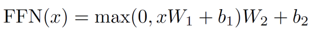
The corresponding implementation in the Annotated Transformer is:

class PositionwiseFeedForward(nn.Module):
    "Implements FFN equation."
    def __init__(self, d_model, d_ff, dropout=0.1):
        super(PositionwiseFeedForward, self).__init__()
        self.w_1 = nn.Linear(d_model, d_ff)
        self.w_2 = nn.Linear(d_ff, d_model)
        self.dropout = nn.Dropout(dropout)

    def forward(self, x):
        return self.w_2(self.dropout(F.relu(self.w_1(x))))

2.3 Encoder Short Summary

The Encoder contains a total of 6 EncoderLayers. Each EncoderLayer consists of 2 sub-layers:

• SubLayer-1 performs Multi-Headed Attention

• SubLayer-2 performs the feedforward neural network

3. The Decoder

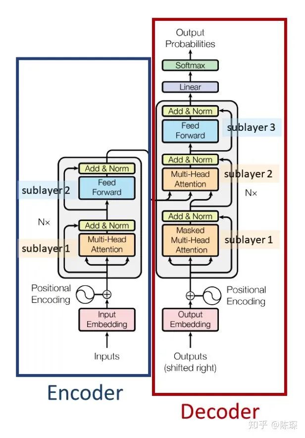
The interaction between the Encoder and Decoder can be understood as:

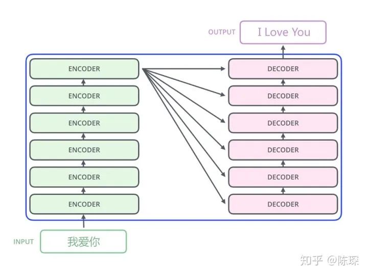
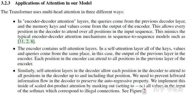
The Decoder is also a stacked structure of N layers. It is divided into 3 sub-layers, and we can see the three main differences between the Encoder and Decoder:

1. Diff_1: Decoder SubLayer-1 uses “masked” Multi-Headed Attention to prevent the model from seeing the data it is supposed to predict, thus preventing leakage.

2. Diff_2: SubLayer-2 is an encoder-decoder multi-head attention.

3. Diff_3: Linear Layer and Softmax Layer are applied to the output of SubLayer-3 to predict the corresponding word probabilities.

3.1 Diff_1: “Masked” Multi-Headed Attention

The goal of the mask is to prevent the decoder from “seeing the future”, similar to preventing students from looking at exam answers. The mask contains 1s and 0s:

The code using the mask in attention is:

if mask is not None:
        scores = scores.masked_fill(mask == 0, -1e9)

To quote the author’s words, “We […] modify the self-attention sub-layer in the decoder stack to prevent positions from attending to subsequent positions. This masking, combined with the fact that the output embeddings are offset by one position, ensures that the predictions for position i can depend only on the known outputs at positions less than i.”

3.2 Diff_2: Encoder-Decoder Multi-Head Attention

The implementation of DecoderLayer in the Annotated Transformer is:

class DecoderLayer(nn.Module):
    "Decoder is made of self-attn, src-attn, and feed forward (defined below)"
    def __init__(self, size, self_attn, src_attn, feed_forward, dropout):
        super(DecoderLayer, self).__init__()
        self.size = size
        self.self_attn = self_attn
        self.src_attn = src_attn
        self.feed_forward = feed_forward
        self.sublayer = clones(SublayerConnection(size, dropout), 3)

    def forward(self, x, memory, src_mask, tgt_mask):
        m = memory
        x = self.sublayer[0](x, lambda x: self.self_attn(x, x, x, tgt_mask))
        x = self.sublayer[1](x, lambda x: self.src_attn(x, m, m, src_mask))
        return self.sublayer[2](x, self.feed_forward)

The key point is that x = self.sublayer1 self.src_attn is an instance of MultiHeadedAttention. query = x, key = m, value = m, mask = src_mask, where x comes from the previous DecoderLayer and m comes from the output of the Encoder.

At this point, we have gathered all three types of Attention in the Transformer:

3.3 Diff_3: Linear and Softmax to Produce Output Probabilities

The final linear layer expands the output of the decoder to the same dimension as the vocabulary size. After softmax, the word with the highest probability is chosen as the prediction result.

Assuming we have a trained network, the prediction steps are as follows:

1. Input the result of the encoder’s entire sentence embedding into the decoder along with a special start symbol </s>. The decoder will produce a prediction, which in our example should be “I”.

2. Input the encoder’s embedding result and “</s>I” into the decoder; at this step, the decoder should predict “Love”.

3. Input the encoder’s embedding result and “</s>I Love” into the decoder; at this step, the decoder should predict “China”.

4. Input the encoder’s embedding result and “</s>I Love China” into the decoder; the decoder should generate the end-of-sentence marker, outputting “</eos>”.

5. Then, the decoder generates </eos>, and the translation is complete.

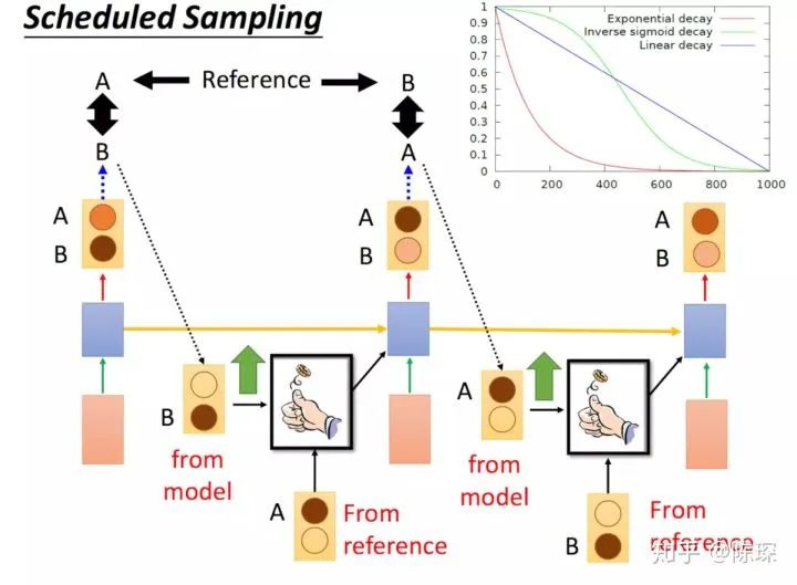
However, during training, if the decoder is not performing well, the predicted words are likely not what we want. If we then feed the incorrect data back into the decoder, it will drift further away:

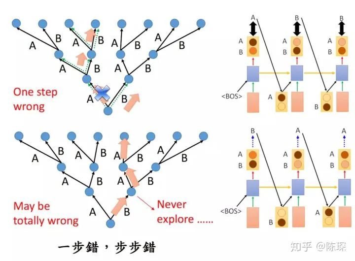
During training, we use “teacher forcing”. We utilize what we know the actual predicted word should be and feed it a correct result as input.

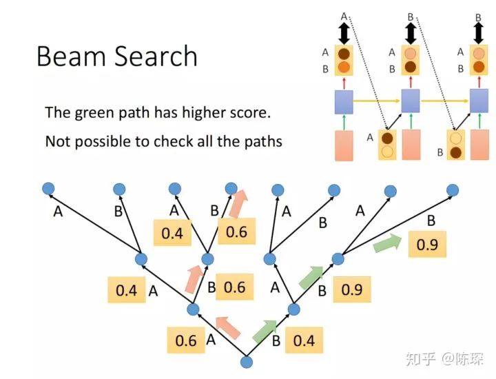
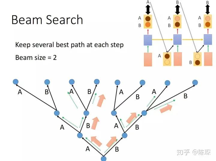
In addition to choosing the highest word (greedy search), there are other options such as “beam search”, which retains multiple predicted words. The Beam Search method no longer just takes one output to train in the next step; we can set a value to take multiple values to train in the next step, where the probability of this path equals the product of the probabilities of each output step. For details, refer to the course by Professor Li Hongyi:

Another method is “Scheduled Sampling”: at first, we only use the actual sentence sequence for training, and as the training progresses, we gradually incorporate the model’s output as input during training.

The corresponding implementation in the Annotated Transformer is:

class Generator(nn.Module):
    "Define standard linear + softmax generation step."
    def __init__(self, d_model, vocab):
        super(Generator, self).__init__()
        self.proj = nn.Linear(d_model, vocab)

    def forward(self, x):
        return F.log_softmax(self.proj(x), dim=-1)

Looking at the figures again, let’s review the structure of the Encoder and Decoder.

References:

• arxiv.org/pdf/1706.0376

• The Transformer: Attention Is All You Need – Glass Box Medicine

• glassboxmedicine.com/20

• jalammar.github.io/illu

• bilibili.com/video/av97

Important! The Natural Language Processing WeChat Academic Group has been established

You can scan the QR code below, and the assistant will invite you to join the group for discussion,

Note: Please modify the remarks when adding, such as [School/Company + Name + Direction]

For example — Harbin Institute of Technology + Zhang San + Dialogue System.

Account owner, please avoid business operations. Thank you!

Recommended Reading:
The Differences and Connections Between Fully Connected Graph Convolutional Networks (GCN) and Self-Attention Mechanisms
Complete Guide to Graph Convolutional Networks (GCN) for Beginners

Paper Appreciation [ACL18] Based on Self-Attentive Constituency Parsing