

Source | Zhihu
Address | https://zhuanlan.zhihu.com/p/47812375
Author | Jian Feng
Editor | WeChat public account on Machine Learning Algorithms and Natural Language Processing
This article is for academic sharing only. If there is any infringement, please contact us to delete the article.
“Attention is All You Need” is a paper that takes the idea of Attention to the extreme, coming from Google. This paper introduces a brand new model called the Transformer, discarding the CNN and RNN used in previous deep learning tasks (although it still uses one-dimensional convolution… ironic). This model is widely applied in the field of NLP, such as machine translation, question answering systems, text summarization, and speech recognition, etc. It can be said to be very powerful.
Today, I intend to try to write about my understanding of the Transformer. The content refers to many summaries from experts.
-
PyTorch implementation of the Transformer model (very well written!)
-
“Attention is All You Need” Simplified Reading (Introduction + Code)
-
Attention Mechanism in Deep Learning – Cloud + Community – Tencent Cloud
-
Attention? Attention!
-
Building the Mighty Transformer for Sequence Tagging in PyTorch
Overall Framework of the Transformer
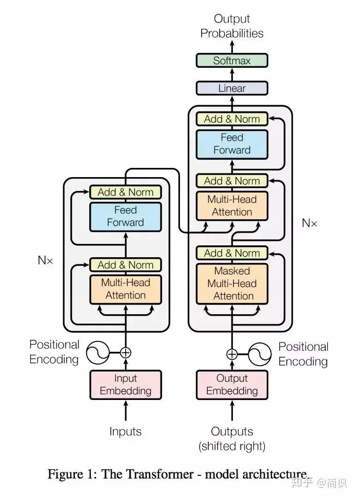
As shown in the figure, at first glance, the architecture of the Transformer seems a bit complex… No worries, let’s explain it slowly…
Similar to the classic seq2seq model, the Transformer model also adopts an encoder-decoder architecture. The left half of the figure, framed by NX, represents one layer of the encoder, and there are a total of 6 such structures in the encoder as mentioned in the paper. The right half of the figure, framed by NX, represents one layer of the decoder, which also has 6 layers.
Define that the input sequence first goes through word embedding, then adds positional encoding before being input into the encoder. The output sequence undergoes the same processing as the input sequence, then is input into the decoder.
Finally, the output of the decoder goes through a linear layer followed by Softmax.
This is the overall framework of the Transformer. Next, let’s introduce the encoder and decoder.
Encoder
The encoder consists of 6 identical layers, each composed of two parts:
-
The first part is multi-head self-attention.
-
The second part is a position-wise feed-forward network, which is a fully connected layer.
Both parts have a residual connection, followed by Layer Normalization.
Decoder
Similar to the encoder, the decoder also consists of 6 identical layers, each including the following three parts:
-
The first part is the multi-head self-attention mechanism.
-
The second part is the multi-head context-attention mechanism.
-
The third part is a position-wise feed-forward network.
Like the encoder, each of the above three parts has a residual connection, followed by a Layer Normalization.
The difference between the decoder and encoder lies in the multi-head context-attention mechanism.
Attention
I mentioned in previous articles that if attention can be described in one sentence, it is that the output of the encoder layer is averaged with weights and then input into the decoder layer. It is mainly used in seq2seq models, and this weighting can be represented by a matrix, also known as the Attention matrix. It indicates the attention on various parts of the input x for a certain moment of output y. This attention is the weighting we just talked about.
Attention is divided into many types, among which two typical ones are additive Attention and multiplicative Attention. Additive Attention directly concatenates the hidden states of the input  and the hidden state of the output
  to obtain
  while multiplicative Attention performs a dot operation on the input and output.
In Google’s paper, the Attention model used is multiplicative Attention.
I wrote a soft-align-attention in my previous article on the ESIM model, which you can refer to for understanding.
Self-Attention
When we talk about the attention mechanism, we often mention two hidden states, namely  and
and  . The former is the hidden state generated at the i-th position of the input sequence, while the latter is the hidden state generated at the t-th position of the output sequence. Self-attention is defined as the output sequence being the same as the input sequence. Therefore, it calculates its own attention scores.
Context-Attention
Context-attention is the attention between the encoder and decoder, differing from self-attention which originates from the same sequence.
Regardless of the type of attention, we can choose many methods to calculate attention weights. Common methods include:
-
Additive attention
-
Local-base
-
General
-
Dot-product
-
Scaled dot-product
The Transformer model uses the last one: scaled dot-product attention.
Scaled Dot-Product Attention
So what is scaled dot-product attention?
Google describes the attention mechanism in the paper as follows:
An attention function can be described as a query and a set of key-value pairs to an output, where the query, keys, values, and output are all vectors. The output is computed as a weighted sum of the values, where the weight assigned to each value is computed by a compatibility of the query with the corresponding key.
The weight distribution of the value is determined by the similarity between the query and the key. The formula in the paper looks like this:

Seeing Q, K, V might be a bit confusing, but don’t worry, it will be explained later.
The only difference between scaled dot-product attention and dot-product attention is that scaled dot-product attention has a scaling factor, called  .
.  represents the dimension of the Key, typically set to 64.
The paper explains the role of  : when
  is large, the result of the dot product becomes large, placing the result in an area where the gradient of the softmax function is very small. Dividing by a scaling factor can somewhat alleviate this situation.
The structure diagram of scaled dot-product attention is shown below.
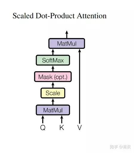
Now let’s explain what K, Q, and V represent:
-
In the self-attention of the encoder, Q, K, and V all come from the same source, which is the output of the previous layer of the encoder. For the first layer of the encoder, they are the inputs obtained by adding the word embedding and positional encoding.
-
In the self-attention of the decoder, Q, K, and V also come from the same source, which is the output of the previous layer of the decoder. For the first layer of the decoder, they are also the inputs obtained by adding the word embedding and positional encoding. However, for the decoder, we do not want it to access the next time step (i.e., future information, we do not want it to see the information it is about to predict), so we need to apply sequence masking.
-
In the encoder-decoder attention, Q comes from the output of the previous layer of the decoder, while K and V come from the output of the encoder, and K and V are the same.
-
The dimensions of Q, K, and V are the same, represented by
 ,
,  , and , respectively.
Currently, the description may be a bit abstract and hard to understand. In some applications, for example, in automatic question answering tasks, Q can represent the word vector sequence of the answer, taking K = V as the word vector sequence of the question, then the output is the so-called Aligned Question Embedding.
One of the main contributions of Google’s paper is that it showed that internal attention is quite important for sequence encoding in machine translation (even in general Seq2Seq tasks), while previous research on Seq2Seq primarily applied the attention mechanism to the decoding end.
Implementation of Scaled Dot-Product Attention
import torch
import torch.nn as nn
import torch.functional as F
import numpy as np

class ScaledDotProductAttention(nn.Module):
    """Scaled dot-product attention mechanism."""

    def __init__(self, attention_dropout=0.0):
        super(ScaledDotProductAttention, self).__init__()
        self.dropout = nn.Dropout(attention_dropout)
        self.softmax = nn.Softmax(dim=2)

    def forward(self, q, k, v, scale=None, attn_mask=None):
        """
        Forward propagation.
        Args:
         q: Queries tensor, shape [B, L_q, D_q]
         k: Keys tensor, shape [B, L_k, D_k]
         v: Values tensor, shape [B, L_v, D_v], generally k
         scale: Scaling factor, a float scalar
         attn_mask: Masking tensor, shape [B, L_q, L_k]
        Returns:
         Context tensor and attention tensor
        """
        attention = torch.bmm(q, k.transpose(1, 2))
        if scale:
            attention = attention * scale
        if attn_mask:
            # Set a negative infinity for places that need masking
            attention = attention.masked_fill_(attn_mask, -np.inf)
	# Calculate softmax
        attention = self.softmax(attention)
	# Add dropout
        attention = self.dropout(attention)
	# Dot product with V
        context = torch.bmm(attention, v)
        return context, attention
Multi-head Attention
Having understood scaled dot-product attention, multi-head attention is also easy to understand. The paper mentions that they found splitting Q, K, and V into h parts after a linear mapping and performing scaled dot-product attention on each part yields better results. Then, the results from each part are combined and passed through a linear mapping again to obtain the final output. This is what is known as multi-head attention. The hyperparameter h above is the number of heads, which is set to 8 by default in the paper.
The structure diagram of multi-head attention is shown below.
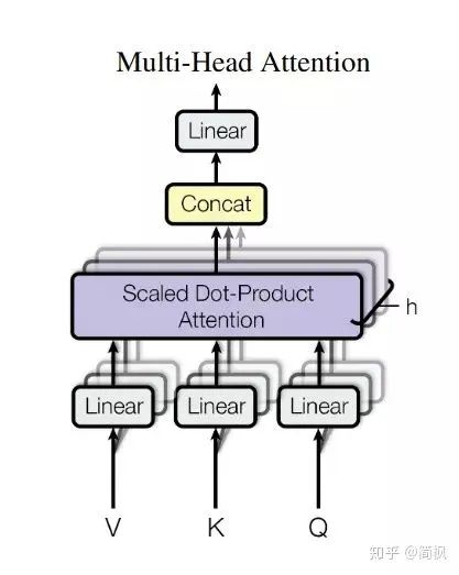
It is worth noting that the splitting mentioned above is done along the dimensions of  , , and . Therefore, the input to the scaled dot-product attention actually equals the input before entering the scaled dot-product attention.
The formula for multi-head attention is as follows:
Where,
In the paper, = 512, h = 8, so in scaled dot-product attention,
It can be seen that multi-head means performing the same operation multiple times, without sharing parameters, and then concatenating the results.
Implementation of Multi-Head Attention
class MultiHeadAttention(nn.Module):

    def __init__(self, model_dim=512, num_heads=8, dropout=0.0):
        super(MultiHeadAttention, self).__init__()

        self.dim_per_head = model_dim // num_heads
        self.num_heads = num_heads
        self.linear_k = nn.Linear(model_dim, self.dim_per_head * num_heads)
        self.linear_v = nn.Linear(model_dim, self.dim_per_head * num_heads)
        self.linear_q = nn.Linear(model_dim, self.dim_per_head * num_heads)

        self.dot_product_attention = ScaledDotProductAttention(dropout)
        self.linear_final = nn.Linear(model_dim, model_dim)
        self.dropout = nn.Dropout(dropout)

        # Layer normalization after multi-head attention
        self.layer_norm = nn.LayerNorm(model_dim)

    def forward(self, key, value, query, attn_mask=None):
	# Residual connection
        residual = query
        dim_per_head = self.dim_per_head
        num_heads = self.num_heads
        batch_size = key.size(0)

        # Linear projection
        key = self.linear_k(key)
        value = self.linear_v(value)
        query = self.linear_q(query)

        # Split by heads
        key = key.view(batch_size * num_heads, -1, dim_per_head)
        value = value.view(batch_size * num_heads, -1, dim_per_head)
        query = query.view(batch_size * num_heads, -1, dim_per_head)

        if attn_mask:
            attn_mask = attn_mask.repeat(num_heads, 1, 1)

        # Scaled dot product attention
        scale = (key.size(-1)) ** -0.5
        context, attention = self.dot_product_attention(
          query, key, value, scale, attn_mask)

        # Concatenate heads
        context = context.view(batch_size, -1, dim_per_head * num_heads)

        # Final linear projection
        output = self.linear_final(context)

        # Dropout
        output = self.dropout(output)

        # Add residual and norm layer
        output = self.layer_norm(residual + output)

        return output, attention
In the code above, the Residual connection has been explained in a previous article, so I will not elaborate further here, only explaining Layer normalization.
Layer Normalization
Normalization has many types, but they all share a common purpose: to transform the input into data with a mean of 0 and a variance of 1. We perform normalization before sending data into the activation function because we do not want the input data to fall into the saturation area of the activation function.
Speaking of normalization, we must mention Batch Normalization.
The main idea of BN is: to normalize the data on each batch of data at every layer. We may normalize the input data, but after passing through the network layer, our data is no longer normalized. As this situation develops, the deviation of data becomes larger, and my backpropagation needs to consider these large deviations, forcing us to use a smaller learning rate to prevent gradient vanishing or exploding.
The specific approach of BN is to normalize on each mini-batch, as shown in the figure below:
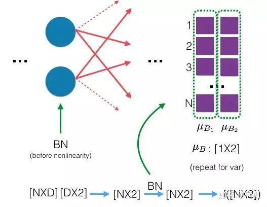
As can be seen, the mean on the right side is calculated along the batch direction N!
The calculation formula for Batch Normalization is as follows:
So what is Layer Normalization? It is also a way to normalize data, but LN calculates the mean and variance on each sample, rather than the mean and variance in the batch direction like BN!
Below is a diagram of Layer Normalization:
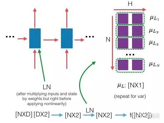
Comparing the above LN diagram with the BN diagram clearly shows the difference between the two!
Next, let’s look at the formula for LN:
Mask
A mask is used to cover certain values so that they do not affect parameter updates. The Transformer model involves two types of masks, namely padding mask and sequence mask.
Among them, the padding mask is used in all scaled dot-product attention, while the sequence mask is only used in the self-attention of the decoder.
Padding Mask
What is padding mask? Since the length of input sequences in each batch is different, we need to align the input sequences. Specifically, this means filling zeros at the end of shorter sequences. Since these padding positions are actually meaningless, our attention mechanism should not focus on these positions, so we need to handle them.
The specific approach is to add a very large negative number (negative infinity) to these positions, so that after softmax, the probabilities of these positions approach 0!
Our padding mask is actually a tensor where each value is a Boolean, with false values indicating the places we need to handle.
Implementation:
def padding_mask(seq_k, seq_q):
    # seq_k and seq_q have the shape [B,L]
    len_q = seq_q.size(1)
    # `PAD` is 0
    pad_mask = seq_k.eq(0)
    pad_mask = pad_mask.unsqueeze(1).expand(-1, len_q, -1)  # shape [B, L_q, L_k]
    return pad_mask
Sequence mask
As mentioned earlier, the sequence mask is used to prevent the decoder from seeing future information. That is, for a sequence, at time step t, the output of our decoder should only rely on the outputs before time t and not on the outputs after time t. Therefore, we need a method to hide the information after t.
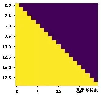
How do we do this? It’s simple: generate an upper triangular matrix with all values in the upper triangle set to 1, the lower triangle set to 0, and the diagonal also set to 0. Applying this matrix to each sequence will achieve our goal.
The specific code implementation is as follows:
def sequence_mask(seq):
    batch_size, seq_len = seq.size()
    mask = torch.triu(torch.ones((seq_len, seq_len), dtype=torch.uint8),
                    diagonal=1)
    mask = mask.unsqueeze(0).expand(batch_size, -1, -1)  # [B, L, L]
    return mask
The effect is as follows:
-
For the self-attention of the decoder, the scaled dot-product attention used inside requires both padding mask and sequence mask as attn_mask, and the specific implementation is to add the two masks to form attn_mask.
-
In other cases, attn_mask is uniformly equal to the padding mask.
Positional Embedding
The current Transformer architecture has not extracted the sequential order of information, which is very important for sequences. If this information is missing, our results might be: all words are correct, but they cannot form meaningful sentences.
To solve this problem, the paper uses Positional Embedding: encoding the positions of words in the sequence.
In implementation, sine and cosine functions are used. The formula is as follows:

Where pos refers to the position of the word in the sequence. As can be seen, at even positions, sine encoding is used, while at odd positions, cosine encoding is used.
From the encoding formula, it can be seen that for a given word position pos, we can encode it into a vector of . This means that each dimension of the position encoding corresponds to a sine curve, where the wavelengths form a geometric sequence from  to .
to .
The above position encoding is absolute position encoding. However, the relative position of words is also very important. This is why the paper uses trigonometric functions!
The sine function can express relative positional information, and the main mathematical basis is the following two formulas:

The above formula indicates that for the positional offset k between vocabulary,  can be expressed as the combination of
  and
and  .
.
Specific implementation is as follows:
class PositionalEncoding(nn.Module):

    def __init__(self, d_model, max_seq_len):
        """Initialization.
        Args:
            d_model: A scalar. The dimension of the model, set to 512 in the paper.
            max_seq_len: A scalar. The maximum length of the text sequence.
        """
        super(PositionalEncoding, self).__init__()

        # Construct the PE matrix according to the formula provided in the paper
        position_encoding = np.array([
          [pos / np.power(10000, 2.0 * (j // 2) / d_model) for j in range(d_model)]
          for pos in range(max_seq_len)])
        # Use sine for even indices, cosine for odd indices
        position_encoding[:, 0::2] = np.sin(position_encoding[:, 0::2])
        position_encoding[:, 1::2] = np.cos(position_encoding[:, 1::2])

        # Add a row of zeros to the PE matrix representing the positional encoding for `PAD`
        # It is often added to word embeddings as well, representing the word embedding for the `UNK`, and the two are quite similar.
        # Why do we need this extra encoding for `PAD`? It's simple, because the lengths of text sequences vary, we need to align them.
        # For shorter sequences, we use 0 to fill at the end; we also need the encoding for these padded positions, which is the positional encoding corresponding to `PAD`.
        pad_row = torch.zeros([1, d_model])
        position_encoding = torch.cat((pad_row, position_encoding))

        # Embedding operation, +1 is because of the addition of the `PAD` encoding position.
        # If the vocabulary increases with `UNK`, we also need to +1. Look, the two are very similar.
        self.position_encoding = nn.Embedding(max_seq_len + 1, d_model)
        self.position_encoding.weight = nn.Parameter(position_encoding,
                                                     requires_grad=False)
    def forward(self, input_len):
        """Forward propagation of the neural network.
        Args:
          input_len: A tensor with shape [BATCH_SIZE, 1]. Each tensor value represents the length of the corresponding text sequence in this batch.
        Returns:
          Returns the positional encoding of this batch of sequences, aligned.
        """
        # Find the maximum length of this batch of sequences
        max_len = torch.max(input_len)
        tensor = torch.cuda.LongTensor if input_len.is_cuda else torch.LongTensor
        # Align the position of each sequence, filling 0 at the end of the original sequence position
        # Here, range starts from 1 to avoid the position of PAD (0)
        input_pos = tensor([
          list(range(1, len + 1)) + [0] * (max_len - len) for len in input_len])
        return self.position_encoding(input_pos)
Position-wise Feed-Forward Network
This is a fully connected network, consisting of two linear transformations and a non-linear function (which is actually just ReLU). The formula is as follows:

This linear transformation behaves the same at different positions and uses different parameters between different layers.
Here, two one-dimensional convolutions are utilized in the implementation.
Implementation is as follows:
class PositionalWiseFeedForward(nn.Module):

    def __init__(self, model_dim=512, ffn_dim=2048, dropout=0.0):
        super(PositionalWiseFeedForward, self).__init__()
        self.w1 = nn.Conv1d(model_dim, ffn_dim, 1)
        self.w2 = nn.Conv1d(ffn_dim, model_dim, 1)
        self.dropout = nn.Dropout(dropout)
        self.layer_norm = nn.LayerNorm(model_dim)

    def forward(self, x):
        output = x.transpose(1, 2)
        output = self.w2(F.relu(self.w1(output)))
        output = self.dropout(output.transpose(1, 2))

        # Add residual and norm layer
        output = self.layer_norm(x + output)
        return output
Implementation of the Transformer
Now we can start building the Transformer model, with 6 layers on both the encoder and decoder sides, implemented as follows, first for the encoder side:
class EncoderLayer(nn.Module):
    """One layer of the Encoder."""

    def __init__(self, model_dim=512, num_heads=8, ffn_dim=2048, dropout=0.0):
        super(EncoderLayer, self).__init__()

        self.attention = MultiHeadAttention(model_dim, num_heads, dropout)
        self.feed_forward = PositionalWiseFeedForward(model_dim, ffn_dim, dropout)

    def forward(self, inputs, attn_mask=None):

        # Self attention
        context, attention = self.attention(inputs, inputs, inputs, padding_mask)

        # Feed forward network
        output = self.feed_forward(context)

        return output, attention


class Encoder(nn.Module):
    """Encoder composed of multiple EncoderLayer."""

    def __init__(self,
               vocab_size,
               max_seq_len,
               num_layers=6,
               model_dim=512,
               num_heads=8,
               ffn_dim=2048,
               dropout=0.0):
        super(Encoder, self).__init__()

        self.encoder_layers = nn.ModuleList(
          [EncoderLayer(model_dim, num_heads, ffn_dim, dropout) for _ in
drange(num_layers)])

        self.seq_embedding = nn.Embedding(vocab_size + 1, model_dim, padding_idx=0)
        self.pos_embedding = PositionalEncoding(model_dim, max_seq_len)

    def forward(self, inputs, inputs_len):
        output = self.seq_embedding(inputs)
        output += self.pos_embedding(inputs_len)

        self_attention_mask = padding_mask(inputs, inputs)

        attentions = []
        for encoder in self.encoder_layers:
            output, attention = encoder(output, self_attention_mask)
            attentions.append(attention)

        return output, attentions
Then for the Decoder side:
class DecoderLayer(nn.Module):

    def __init__(self, model_dim, num_heads=8, ffn_dim=2048, dropout=0.0):
        super(DecoderLayer, self).__init__()

        self.attention = MultiHeadAttention(model_dim, num_heads, dropout)
        self.feed_forward = PositionalWiseFeedForward(model_dim, ffn_dim, dropout)

    def forward(self,
              dec_inputs,
              enc_outputs,
              self_attn_mask=None,
              context_attn_mask=None):
        # Self attention, all inputs are decoder inputs
        dec_output, self_attention = self.attention(
          dec_inputs, dec_inputs, dec_inputs, self_attn_mask)

        # Context attention
        # Query is decoder's outputs, key and value are encoder's inputs
        dec_output, context_attention = self.attention(
          enc_outputs, enc_outputs, dec_output, context_attn_mask)

        # Decoder's output, or context
        dec_output = self.feed_forward(dec_output)

        return dec_output, self_attention, context_attention


class Decoder(nn.Module):

    def __init__(self,
               vocab_size,
               max_seq_len,
               num_layers=6,
               model_dim=512,
               num_heads=8,
               ffn_dim=2048,
               dropout=0.0):
        super(Decoder, self).__init__()

        self.num_layers = num_layers

        self.decoder_layers = nn.ModuleList(
          [DecoderLayer(model_dim, num_heads, ffn_dim, dropout) for _ in
drange(num_layers)])

        self.seq_embedding = nn.Embedding(vocab_size + 1, model_dim, padding_idx=0)
        self.pos_embedding = PositionalEncoding(model_dim, max_seq_len)

    def forward(self, inputs, inputs_len, enc_output, context_attn_mask=None):
        output = self.seq_embedding(inputs)
        output += self.pos_embedding(inputs_len)

        self_attention_padding_mask = padding_mask(inputs, inputs)
        seq_mask = sequence_mask(inputs)
        self_attn_mask = torch.gt((self_attention_padding_mask + seq_mask), 0)

        self_attentions = []
        context_attentions = []
        for decoder in self.decoder_layers:
            output, self_attn, context_attn = decoder(
            output, enc_output, self_attn_mask, context_attn_mask)
            self_attentions.append(self_attn)
            context_attentions.append(context_attn)

        return output, self_attentions, context_attentions
Combining them gives us the Transformer model.
class Transformer(nn.Module):

    def __init__(self,
               src_vocab_size,
               src_max_len,
               tgt_vocab_size,
               tgt_max_len,
               num_layers=6,
               model_dim=512,
               num_heads=8,
               ffn_dim=2048,
               dropout=0.2):
        super(Transformer, self).__init__()

        self.encoder = Encoder(src_vocab_size, src_max_len, num_layers, model_dim,
                               num_heads, ffn_dim, dropout)
        self.decoder = Decoder(tgt_vocab_size, tgt_max_len, num_layers, model_dim,
                               num_heads, ffn_dim, dropout)

        self.linear = nn.Linear(model_dim, tgt_vocab_size, bias=False)
        self.softmax = nn.Softmax(dim=2)

    def forward(self, src_seq, src_len, tgt_seq, tgt_len):
        context_attn_mask = padding_mask(tgt_seq, src_seq)

        output, enc_self_attn = self.encoder(src_seq, src_len)

        output, dec_self_attn, ctx_attn = self.decoder(
          tgt_seq, tgt_len, output, context_attn_mask)

        output = self.linear(output)
        output = self.softmax(output)

        return output, enc_self_attn, dec_self_attn, ctx_attn
That’s all!
GitHub address: pengshuang/Transformer
Important! The WeChat group for Natural Language Processing – Academic Exchange has been established.
You can scan the QR code below, and the assistant will invite you to join the group for discussion.
Note: Please modify the note to [School/Company + Name + Field] when adding.
For example – HIT + Zhang San + Dialogue System.
The account owner, please avoid adding if you are a sales representative. Thank you!


Recommended Reading:
The Differences and Connections between Fully Connected Graph Convolutional Networks (GCN) and Self-Attention Mechanisms
Complete Guide for Beginners on Graph Convolutional Networks (GCN)

Paper Review [ACL18] Component Syntax Analysis Based on Self-Attentive