Understanding LSTM and GRU Gating Mechanisms in Three Simplifications

Machine Heart Column

Author:Zhang Hao

RNNs are very successful in handling sequential data. However, understanding RNNs and their variants, LSTM and GRU, remains a challenging task. This article introduces a simple and universal method for understanding LSTM and GRU. By simplifying the mathematical formalization of LSTM and GRU three times, we can visualize the data flow in a single diagram, which allows for a concise and intuitive understanding and analysis of the underlying principles. Moreover, the analysis method of simplifying to a single diagram has universality and can be widely used for the analysis of other gated networks.

1. RNN, Gradient Explosion, and Gradient Vanishing

1.1 RNN

In recent years, deep learning models have been very effective in handling data with very complex internal structures. For example, the 2D spatial relationship between pixels in image data is very important, and CNNs (Convolutional Neural Networks) handle this spatial relationship effectively. For sequential data, the temporal relationship between variable-length input sequences is crucial, and RNNs (Recurrent Neural Networks) handle this temporal relationship effectively.

We use the subscript t to denote different positions in the input sequential series, h_t to represent the hidden state vector of the system at time t, and x_t to represent the input at time t. The hidden state vector h_t at time t depends on the current word x_t and the hidden state vector h_(t-1) from the previous moment:

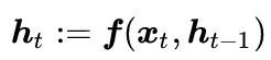
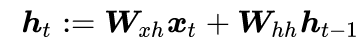
where f is a nonlinear mapping function. A common practice is to calculate the linear transformation of x_t and h_(t-1) followed by a nonlinear activation function, for example,

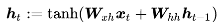
where W_(xh) and W_(hh) are learnable parameter matrices, and the activation function tanh is applied independently to each element of its input.

To visualize the computation process of RNN, we can draw the following diagram:

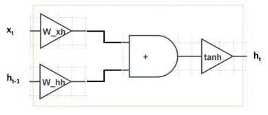
On the left side of the diagram is the input x_t and h_(t-1), and on the right side is the output h_t. The computation proceeds from left to right, and the entire operation consists of three steps: the inputs x_t and h_(t-1) are multiplied by W_(xh) and W_(hh), added together, and passed through the tanh nonlinear transformation.

We can think of h_t as storing the memory in the network; the goal of RNN training is to ensure that h_t records the input information x_1, x_2,…, x_t before time t. After the new word x_t is input into the network, the previous hidden state vector h_(t-1) is transformed into h_t, which is related to the current input x_t.

1.2 Gradient Explosion and Gradient Vanishing

Although RNNs can theoretically capture long-distance dependencies, in practice, they face two challenges: gradient explosion and gradient vanishing.

Consider a simple case where the activation function is an identity transformation; at this point,

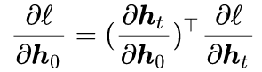
During error backpropagation, when we know the derivative of the loss functionwith respect to the hidden state vector h_t at time t, using the chain rule, we compute the derivative of the loss functionwith respect to the hidden state vector h_0 at time t

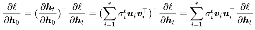
We can utilize the dependency of RNN along the time dimension to calculate

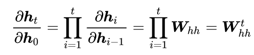
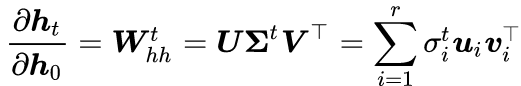
In other words, during error backpropagation, we need to repeatedly multiply by the parameter matrix W_(hh). We perform singular value decomposition (SVD) on the matrix W_(hh)

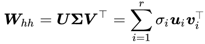
where r is the rank of the matrix W_(hh). Therefore,

The final goal we need to compute is

When t is large, the derivative depends on the largest singular value of the matrix W_(hh)being greater than or less than 1, resulting in either a very large or very small outcome:

(1). Gradient Explosion. When > 1,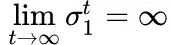then

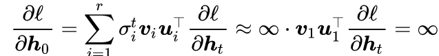
At this time, the derivativewill become very large, resulting in NaN errors during training, affecting convergence, and even causing the network to not converge. This is akin to trying to sell domestic products in other countries, only to find that after numerous tariffs, the price has become so high that the local population cannot afford it. In RNNs, the gradient (derivative) is like the price, which increases as we move forward. This phenomenon is called gradient explosion.

Gradient explosion is relatively easier to handle and can be resolved using gradient clipping:

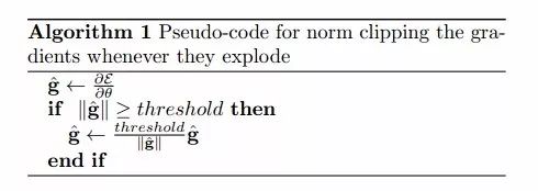
This is like setting a maximum market price regardless of how many tariffs are added, ensuring that the local population can afford it. In RNNs, regardless of how large the gradient is during backpropagation, a threshold can be set to limit the maximum size of the gradient.

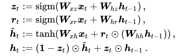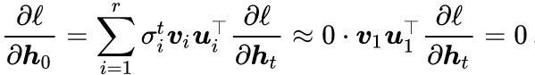(2). Gradient Vanishing. When < 1,then

At this time, the derivativewill become very close to 0, resulting in little difference before and after gradient updates, which diminishes the network’s ability to capture long-term dependencies. This is akin to sending supplies to the front lines in a war; if the supply point is too far from the front, the supplies may be consumed before they arrive. In RNNs, the gradient (derivative) is like food, which is gradually consumed as we move forward. This phenomenon is called gradient vanishing.

The gradient vanishing phenomenon is much harder to address, and how to mitigate gradient vanishing is a key research area for RNNs and almost all other deep learning methods. LSTM and GRU use gate mechanisms to control the flow of information in RNNs to alleviate the gradient vanishing problem. The core idea is to selectively process inputs. For example, when we read a review of a product

Amazing! This box of cereal gave me a perfectly balanced breakfast, as all things should be. I only ate half of it but will definitely be buying again!

we focus on certain words and process them

Amazing! This box of cereal gave me a perfectly balanced breakfast, as all things should be. I only ate half of it but will definitely be buying again!

LSTM and GRU selectively ignore some words, preventing them from participating in the update of the hidden state vector, ultimately retaining only the relevant information for prediction.

2. LSTM

2.1 Mathematical Formalization of LSTM

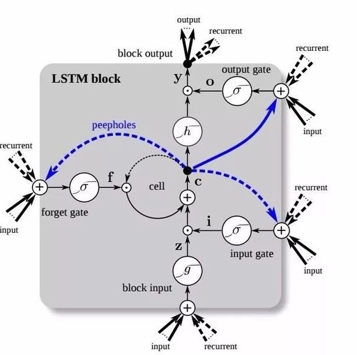
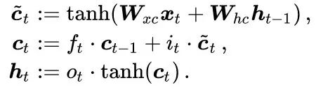
LSTM (Long Short-Term Memory) was proposed by Hochreiter and Schmidhuber, and its mathematical formalization is as follows:

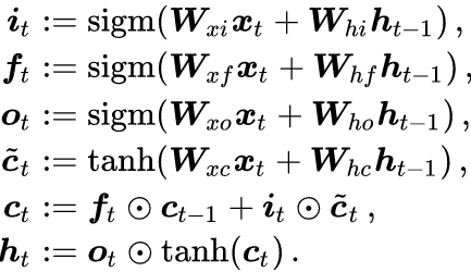
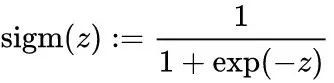
whererepresents element-wise multiplication, and sigm represents the sigmoid function

Compared to RNNs, LSTM has an additional hidden state variable c_t, known as the cell state, used to record information.

This formula may seem quite complex, so to better understand the mechanism of LSTM, many people use diagrams to describe the computation process of LSTM. For example, the following diagram:

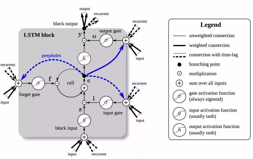
After viewing this, do you still feel confused about LSTM? This is because these diagrams attempt to present all the details of LSTM at once, which can be overwhelming and leave you unsure where to start.

2.2 Three Simplifications to One Diagram

Therefore, the method proposed in this article aims to simplify the unimportant parts of the gating mechanism to focus more on the core ideas of LSTM. The entire process is three simplifications to one diagram, with the following specific steps:

(1). First Simplification: Ignore the Sources of Gating Units i_t, f_t, o_t. The calculation method for the three gating units is completely the same; they are all obtained from the input through linear mapping, with the only difference being the parameters used in the calculations:

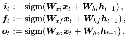
The purpose of using the same calculation method is that they all play a gating role, while using different parameters allows for independent updates of the three gating units during error backpropagation. To simplify the understanding of how LSTM operates, we will not label the computation process of the three gating units in the diagram and assume that they are given.

(2). Second Simplification: Consider One-Dimensional Gating Units i_t, f_t, o_t. In LSTM, each dimension is gated independently, so for simplicity and understanding, we only need to consider the one-dimensional case. After understanding the principles of LSTM, extending from one dimension to multiple dimensions is straightforward. After these two simplifications, the mathematical form of LSTM is reduced to the following three lines

Since the gating units have become one-dimensional, the symbol for element-wise multiplication between vectors has changed to a scalar and vector multiplication ·.

(3). Third Simplification: Binary Outputs of Each Gating Unit. The outputs of the gating units i_t, f_t, o_t range from [0, 1] due to the sigmoid activation function. The purpose of using the sigmoid activation function is to approximate the 0/1 step function, allowing for smooth differentiation based on error backpropagation.

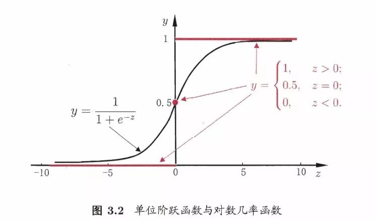
Since the sigmoid activation function aims to approximate the 0/1 step function, for ease of understanding in LSTM analysis, we will consider the gating units to have binary outputs {0, 1}, meaning that the gating units act as switches in a circuit, controlling the flow of information.

(4). One Diagram. The results of the three simplifications are represented in a circuit diagram, with inputs on the left and outputs on the right. In LSTM, one important point to note is that the cell state c_t essentially plays the role of the hidden unit h_t in RNNs, which is often not mentioned in other literature. Therefore, the inputs to the entire diagram are x_t and c_{t-1}, rather than x_t and h_(t-1). For ease of drawing, we need to make final adjustments to the formulas

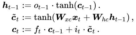
The final result is as follows:

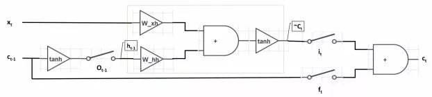
Similar to RNNs, the network takes two inputs and produces one output. It utilizes two parameter matrices W_(xc) and W_(hc), along with the tanh activation function. The difference is that in LSTM, the interaction of information is controlled by three gating units i_t, f_t, o_t. When i_t=1 (switch closed), f_t=0 (switch open), and o_t=1 (switch closed), LSTM degrades to a standard RNN.

2.3 Analysis of Each Unit’s Role in LSTM

Based on this diagram, we can analyze the role of each unit in LSTM:

• Output Gate o_(t-1): The purpose of the output gate is to produce the hidden unit h_(t-1) from the cell state c_(t-1). Not all information in c_(t-1) is relevant to the hidden unit h_(t-1); c_(t-1) may contain much information that is not useful for h_(t-1). Therefore, the role of o_t is to determine which parts of c_(t-1) are useful for h_(t-1) and which parts are not.

• Input Gate i_t: i_t controls the incorporation of the current word x_t into the cell state c_t. In understanding a sentence, the current word x_t may be very important to the overall meaning, or it may not be important at all. The purpose of the input gate is to assess the importance of the current word x_t to the overall context. When the i_t switch is open, the network will not consider the current input x_t.

• Forget Gate f_t: f_t controls the incorporation of the information from the previous cell state c_(t-1) into the cell state c_t. In understanding a sentence, the current word x_t may continue the meaning of the previous context or start describing new content unrelated to the previous context. Unlike the input gate i_t, f_t does not assess the importance of the current word x_t; rather, it assesses the importance of the previous cell state c_(t-1) in computing the current cell state c_t. When the f_t switch is open, the network will not consider the previous cell state c_(t-1).

• Cell State c_t: c_t integrates information from the current word x_t and the previous cell state c_(t-1). This is quite similar to the residual approximation idea in ResNet; through the “shortcut connection” from c_(t-1) to c_t, gradients can be effectively backpropagated. When f_t is closed, the gradient of c_t can be directly transmitted along this shortcut without being affected by the parameters W_(xh) and W_(hh), which is key to LSTM’s effectiveness in alleviating the gradient vanishing phenomenon.

3. GRU

3.1 Mathematical Formalization of GRU

GRU is another mainstream derivative of RNNs. Both RNNs and LSTMs are designed to alleviate the gradient vanishing problem, but their network structures differ. The mathematical formalization of GRU is as follows:

3.2 Three Simplifications to One Diagram

To understand the design philosophy of GRU, we will again apply the method of three simplifications to one diagram:

(1). First Simplification: Ignore the Sources of Gating Units z_t and r_t.

(2). Consider One-Dimensional Gating Units z_t and r_t. After these two simplifications, the mathematical form of GRU is reduced to the following two lines

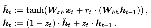
(3). Third Simplification: Binary Outputs of Each Gating Unit. Here, unlike LSTM, when z_t=1, h_t = h_(t-1); when z_t=0, h_t =. Therefore, z_t acts as a single switch.

(4). One Diagram. The results of the three simplifications are represented in a circuit diagram, with inputs on the left and outputs on the right.

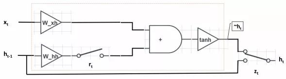
Compared to LSTM, GRU merges the input gate i_t and the forget gate f_t into a single update gate z_t, and it combines the cell state c_t with the hidden unit h_t. When r_t=1 (switch closed) and z_t=0 (switch connected above), GRU degrades to a standard RNN.

3.3 Analysis of Each Unit’s Role in GRU

Based on this diagram, we can analyze the role of each unit in GRU:

• Reset Gate r_t: r_t controls the influence of the previous hidden unit h_(t-1) on the current word x_t. If h_(t-1) is not important for x_t, meaning that the current word x_t begins a new description unrelated to the previous context, then the r_t switch can be opened, allowing h_(t-1) to have no effect on x_t.

• Update Gate z_t: z_t determines whether to ignore the current word x_t. Similar to the input gate i_t in LSTM, z_t assesses the importance of the current word x_t in conveying the overall meaning. When the z_t switch connects to the lower branch, we will ignore the current word x_t, forming a shortcut connection from h_(t-1) to h_t, which allows gradients to be effectively backpropagated. Like LSTM, this shortcut mechanism effectively alleviates the gradient vanishing phenomenon, similar to highway networks.

4. Conclusion

Despite the significant structural differences among RNNs, LSTMs, and GRUs, their basic computation units are consistent; they all perform a linear mapping of x_t and h_t followed by a tanh activation function, as seen in the red boxed portions of the three diagrams. Their differences lie in how they design additional gating mechanisms to control the propagation of gradient information to mitigate the gradient vanishing phenomenon. LSTM uses three gates, GRU uses two; can we reduce this further? MGU (Minimal Gate Unit) attempts to answer this question, featuring only one gating unit. Finally, here’s a small exercise: based on the examples of LSTM and GRU, can you analyze MGU using the three simplifications to one diagram method?

References

1. Yoshua Bengio, Patrice Y. Simard, and Paolo Frasconi. Learning long-term dependencies with gradient descent is difficult. IEEE Transactions on Neural Networks 5(2): 157-166, 1994.

2. Kyunghyun Cho, Bart van Merrienboer, Çaglar Gülçehre, Dzmitry Bahdanau, Fethi Bougares, Holger Schwenk, and Yoshua Bengio. Learning phrase representations using RNN encoder-decoder for statistical machine translation. In EMNLP, pages 1724-1734, 2014.

3. Junyoung Chung, Çaglar Gülçehre, KyungHyun Cho, and Yoshua Bengio. Empirical evaluation of gated recurrent neural networks on sequence modeling. In NIPS Workshop, pages 1-9, 2014.

4. Felix Gers. Long short-term memory in recurrent neural networks. PhD Dissertation, Ecole Polytechnique Fédérale de Lausanne, 2001.

5. Ian J. Goodfellow, Yoshua Bengio, and Aaron C. Courville. Deep learning. Adaptive Computation and Machine Learning, MIT Press, ISBN 978-0-262-03561-3, 2016.

6. Alex Graves. Supervised sequence labelling with recurrent neural networks. Studies in Computational Intelligence 385, Springer, ISBN 978-3-642-24796-5, 2012.

7. Klaus Greff, Rupesh Kumar Srivastava, Jan Koutník, Bas R. Steunebrink, and Jürgen Schmidhuber. LSTM: A search space odyssey. IEEE Transactions on Neural Networks and Learning Systems. 28(10): 2222-2232, 2017.

8. Kaiming He, Xiangyu Zhang, Shaoqing Ren, and Jian Sun. Deep residual learning for image recognition. In CVPR, pages 770-778, 2016.

9. Kaiming He, Xiangyu Zhang, Shaoqing Ren, and Jian Sun. Identity mappings in deep residual networks. In ECCV, pages 630-645, 2016.

10. Sepp Hochreiter and Jürgen Schmidhuber. Long short-term memory. Neural Computation 9(8): 1735-1780, 1997.

11. Rafal Józefowicz, Wojciech Zaremba, and Ilya Sutskever. An empirical exploration of recurrent network architectures. In ICML, pages 2342-2350, 2015.

12. Zachary Chase Lipton. A critical review of recurrent neural networks for sequence learning. CoRR abs/1506.00019, 2015.

13. Razvan Pascanu, Tomas Mikolov, and Yoshua Bengio. On the difficulty of training recurrent neural networks. In ICML, pages 1310-1318, 2013.

14. Rupesh Kumar Srivastava, Klaus Greff, and Jürgen Schmidhuber. Highway networks. In ICML Workshop, pages 1-6, 2015.

15. Guo-Bing Zhou, Jianxin Wu, Chen-Lin Zhang, and Zhi-Hua Zhou. Minimal gated unit for recurrent neural networks. International Journal of Automation and Computing, 13(3): 226-234, 2016.

This article is part of the Machine Heart column; please contact this public account for authorization to reprint

✄————————————————

Join Machine Heart (Full-time Reporter / Intern): [email protected]

Submissions or Reporting Inquiries: content@jiqizhixin.com

Advertising & Business Cooperation: [email protected]