LSTM Neural Network Time Series Prediction

Given a simple dataset, we use Long Short-Term Memory (LSTM) neural networks to implement time series prediction, with the ReLU function as the activation function. The implementation code is as follows:

Part 1. Time Series Prediction Implementation

% LSTM Neural Network Time Series Prediction
clear,clc
res = xlsread('dataset.xlsx');
temp = randperm(103);

P_train = res(temp(1: 80), 1: 7)';
T_train = res(temp(1: 80), 8)';
M = size(P_train, 2);

P_test = res(temp(81: end), 1: 7)';
T_test = res(temp(81: end), 8)';
N = size(P_test, 2);

[P_train, ps_input] = mapminmax(P_train, 0, 1);
P_test = mapminmax('apply', P_test, ps_input);

t_train, ps_output] = mapminmax(T_train, 0, 1);
t_test = mapminmax('apply', T_test, ps_output);

P_train =  double(reshape(P_train, 7, 1, 1, M));
P_test  =  double(reshape(P_test , 7, 1, 1, N));

t_train = t_train';
t_test  = t_test' ;

for i = 1 : M
    p_train{i, 1} = P_train(:, :, 1, i);
end

for i = 1 : N
    p_test{i, 1}  = P_test( :, :, 1, i);
end

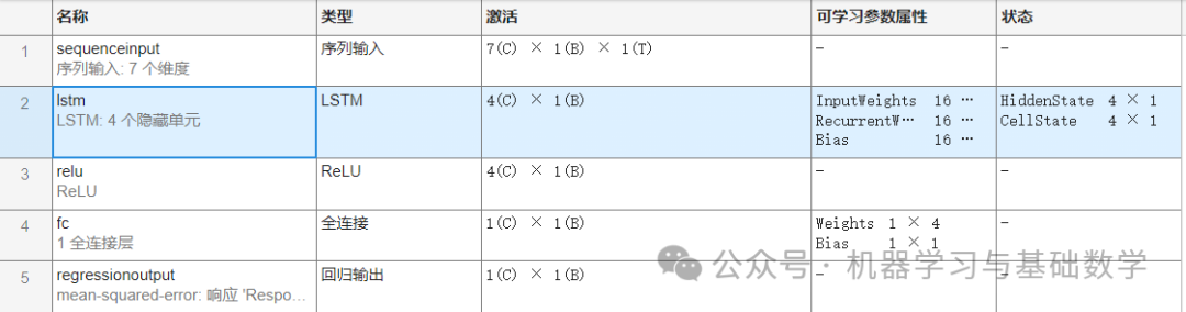
layers = [
    sequenceInputLayer(7)              
    lstmLayer(4, 'OutputMode', 'last') 
    reluLayer                            
    fullyConnectedLayer(1)             
    regressionLayer];                  
 
options = trainingOptions('adam', ...    
    'MaxEpochs', 1500, ...               
    'InitialLearnRate', 0.01, ...         
    'LearnRateSchedule', 'piecewise', ... 
    'LearnRateDropFactor', 0.1, ...       
    'LearnRateDropPeriod', 1200, ...      
    'Shuffle', 'every-epoch', ...          
    'Plots', 'training-progress', ...      
    'Verbose', false);

net = trainNetwork(p_train, t_train, layers, options);
t_sim1 = predict(net, p_train);
t_sim2 = predict(net, p_test );
T_sim1 = mapminmax('reverse', t_sim1, ps_output);
T_sim2 = mapminmax('reverse', t_sim2, ps_output);

error1 = sqrt(sum((T_sim1' - T_train).^2) ./ M);
error2 = sqrt(sum((T_sim2' - T_test ).^2) ./ N);
analyzeNetwork(net)

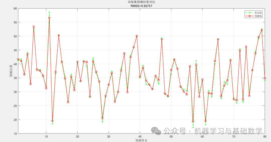
figure
plot(1: M, T_train, 'g--+', 1: M, T_sim1, 'r-o', 'LineWidth', 1)
legend('True Values', 'Predicted Values')
xlabel('Predicted Samples')
ylabel('Prediction Results')
string = {'Training Set Prediction Results Comparison'; ['RMSE=' num2str(error1)]};
title(string)
xlim([1, M])
grid

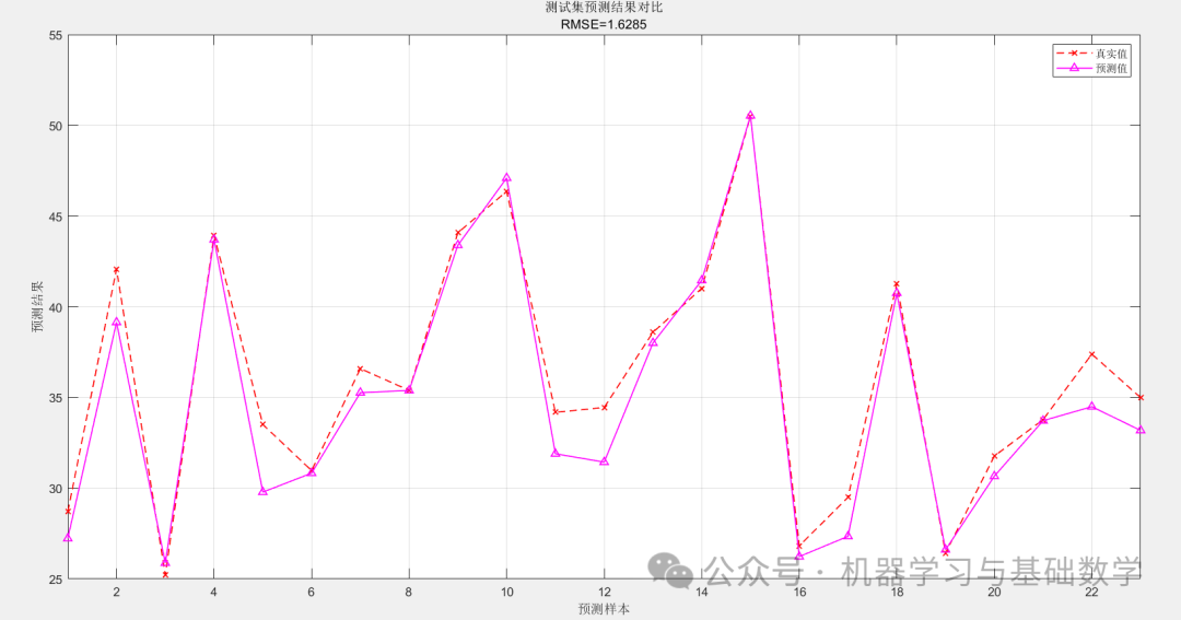
figure
plot(1: N, T_test, 'r--x', 1: N, T_sim2, 'm-^', 'LineWidth', 1)
legend('True Values', 'Predicted Values')
xlabel('Predicted Samples')
ylabel('Prediction Results')
string = {'Test Set Prediction Results Comparison'; ['RMSE=' num2str(error2)]};
title(string)
xlim([1, N])
grid

R1 = 1 - norm(T_train - T_sim1')^2 / norm(T_train - mean(T_train))^2;
R2 = 1 - norm(T_test  - T_sim2')^2 / norm(T_test  - mean(T_test ))^2;

disp(['Training Set R2:', num2str(R1)])
disp(['Test Set R2:', num2str(R2)])

mae1 = sum(abs(T_sim1' - T_train)) ./ M ;
mae2 = sum(abs(T_sim2' - T_test )) ./ N ;

disp(['Training Set MAE:', num2str(mae1)])
disp(['Test Set MAE:', num2str(mae2)])

mbe1 = sum(T_sim1' - T_train) ./ M ;
mbe2 = sum(T_sim2' - T_test ) ./ N ;

disp(['Training Set MBE:', num2str(mbe1)])
disp(['Test Set MBE:', num2str(mbe2)])

sz = 25;
c = 'r';

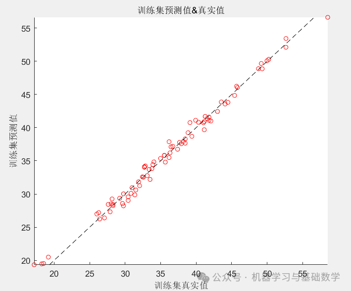
figure
scatter(T_train, T_sim1, sz, c)
hold on
plot(xlim, ylim, '--k')
xlabel('Training Set True Values');
ylabel('Training Set Predicted Values');
xlim([min(T_train) max(T_train)])
ylim([min(T_sim1) max(T_sim1)])
title('Training Set Predicted Values & True Values')

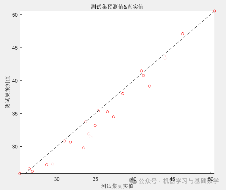
figure
scatter(T_test, T_sim2, sz, c)
hold on
plot(xlim, ylim, '--k')
xlabel('Test Set True Values');
ylabel('Test Set Predicted Values');
xlim([min(T_test) max(T_test)])
ylim([min(T_sim2) max(T_sim2)])
title('Test Set Predicted Values & True Values')

Happy New Year

Happy Spring Festival

Part 2. Plotting Results Display

Part 2. Resource Acquisition:

For those who need it, please reply with the keyword 【MATLAB Time Series Prediction 1.25】 in the background to download it yourself!

Follow our public account 【Machine Learning and Basic Mathematics】 for more valuable knowledge!