Click the "Learn Visuals" above, and select to add "Star" or "Pin to Top".

Important resources delivered to you first.
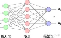
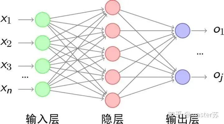
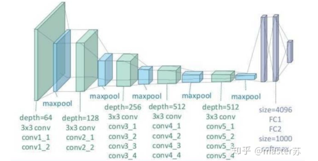
Author on Zhihu | masterSuLink | https://zhuanlan.zhihu.com/p/139617364This article is about 3200 words, recommended reading time 5 minutesThis article introduces the visualization of the LSTM model structure.Recently, I have been learning about the application of LSTM in time series prediction, but I encountered a significant problem: after adding time steps to the traditional BP network, its structure becomes difficult to understand, and its input-output data format is also hard to grasp. There are many articles online introducing the LSTM structure, but they are not intuitive and very unfriendly to beginners. I also pondered for a long time and only understood the secrets after looking at many materials and LSTM structure diagrams shared by netizens. The content of this article is as follows:1. Traditional BP networks and CNN networks2. LSTM networks3. Input structure of LSTM4. LSTM in PyTorch4.1 LSTM model defined in PyTorch4.2 Data format fed to LSTM4.3 Output format of LSTM5. LSTM combined with other networksTraditional BP Networks and CNN NetworksBP networks and CNN networks do not have a time dimension and are not much different from traditional machine learning algorithms. CNN can also be understood as stacking multiple layers when processing the three channels of color images. The three-dimensional matrix of the image can be regarded as spatial slices. When writing code, just follow the diagram and stack them layer by layer. The following diagram shows a typical BP network and CNN network.BP NetworkCNN NetworkThe hidden layers, convolutional layers, pooling layers, fully connected layers, etc. in the diagram are all actual existing layers, stacked layer by layer, which is easy to understand in space. Therefore, when writing code, it is basically just looking at the diagram to write code. For example, using Keras:
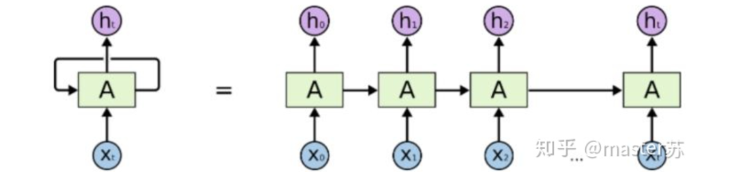
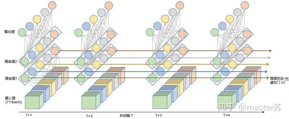
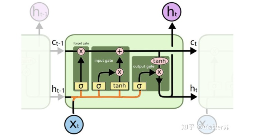
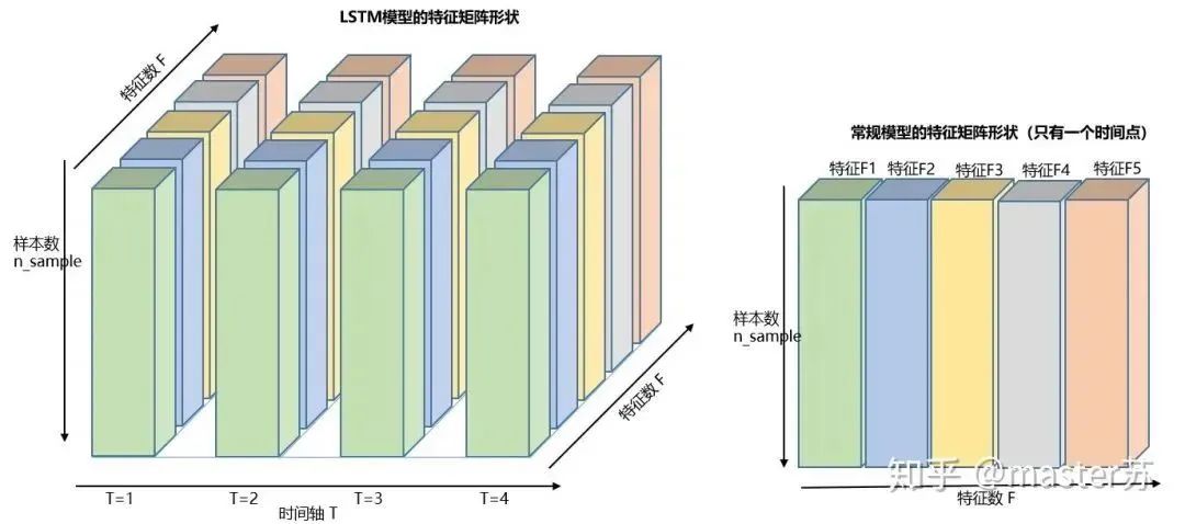
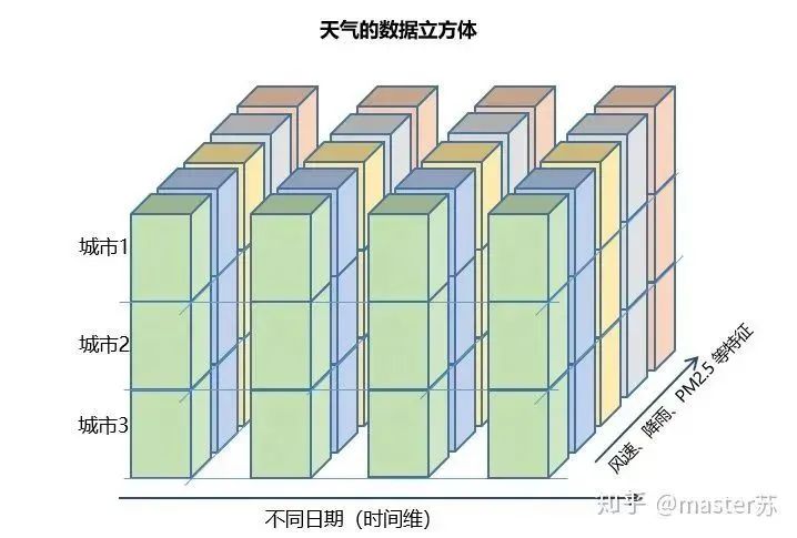
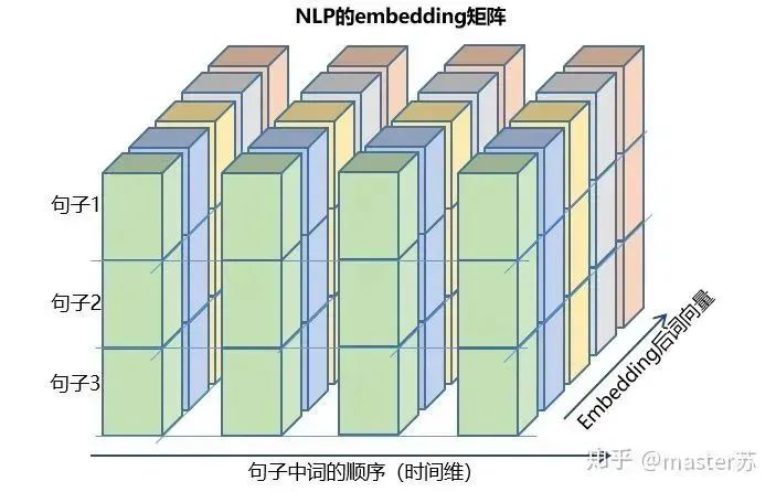
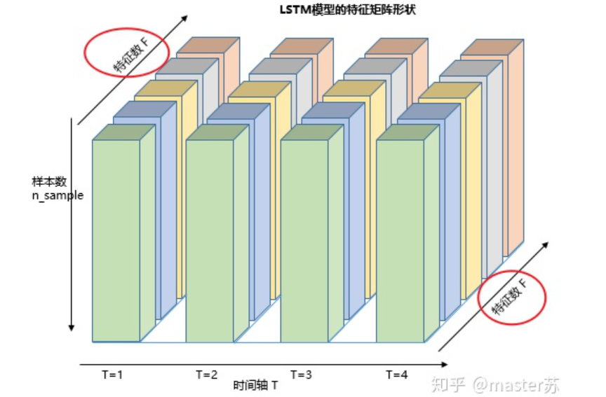
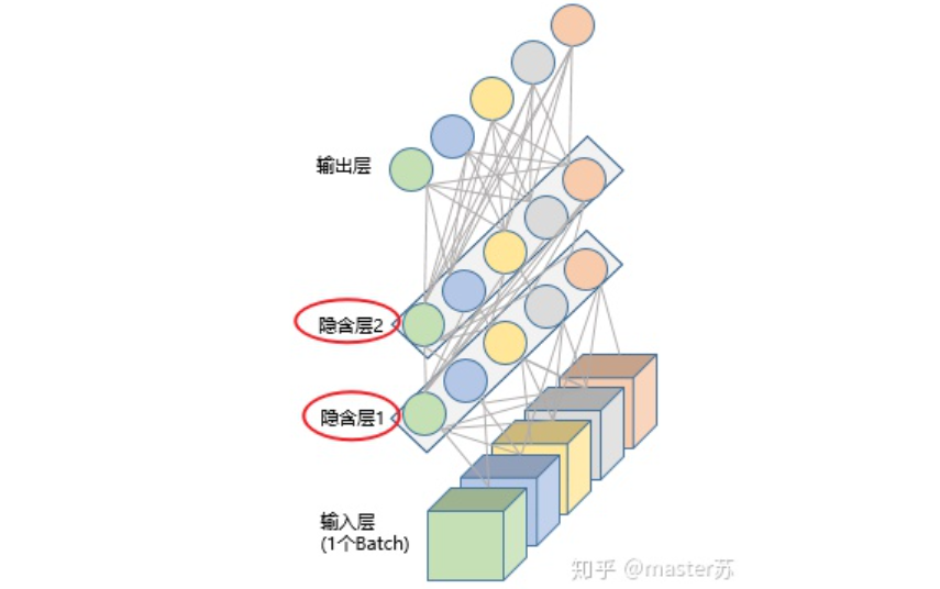
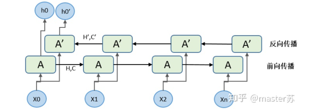
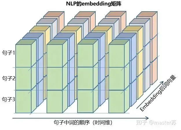
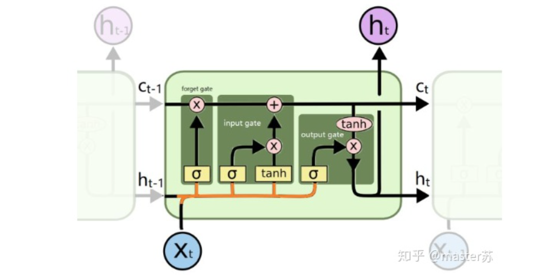
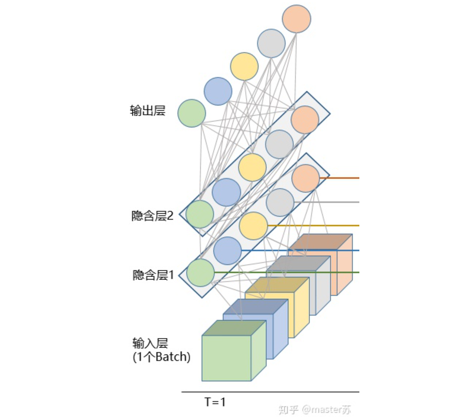
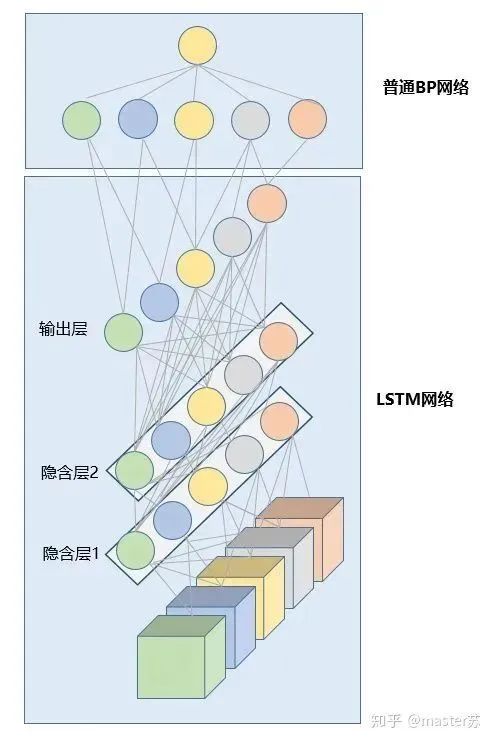
LSTM NetworksWhen we search for LSTM structures online, the most common image we see is the one below:RNN NetworkThis is the classic structure diagram of the RNN recurrent neural network. LSTM is just an improvement on the hidden layer node A, and the overall structure remains unchanged. Therefore, this article also discusses the visualization of this structure.The middle A node hidden layer indicates that the left side represents an LSTM network with only one hidden layer. The so-called LSTM recurrent neural network is a cyclic utilization on the time axis. When unfolded on the time axis, it results in the right diagram.Looking at the left diagram, many students think that LSTM is a single input, single output network structure with only one hidden neuron. Looking at the right diagram, they think that LSTM has multiple inputs and outputs, with multiple hidden neurons. The number of A nodes represents the number of hidden layer nodes.WTH? It’s hard to wrap my head around this. This is the thinking of traditional networks and spatial structures.In fact, in the right diagram, we see Xt representing the sequence, where the subscript t is the time axis. Therefore, the number of A nodes represents the length of the time axis, which is the state (Ht) of the same neuron at different moments, not the number of hidden layer neurons.We know that the LSTM network uses the information from the previous moment, combined with the input information from the current moment, to train together.For example: On the first day, I got sick (initial state H0), then took medicine (using input information X1 to train the network), on the second day I felt better but not completely well (H1), took medicine again (X2), and my condition improved (H2), and so on until I recovered. Therefore, the input Xt is taking medicine, the time axis T is the number of days taking medicine, and the hidden layer state is the condition of the illness. Therefore, I am still me, just different states of me.In fact, the LSTM network is like this:LSTM Network StructureThe above diagram represents an LSTM network with 2 hidden layers. When viewed at T=1, it is a typical BP network, and when viewed at T=2, it is also a typical BP network. However, when unfolded along the time axis, the hidden layer information H, C trained at T=1 will be passed to the next moment T=2, as shown in the diagram below. The five common arrows pointing right in the above diagram also represent the transmission of hidden layer states along the time axis.Note that H in the diagram represents the hidden layer state, and C is the forget gate. We will explain their dimensions later.Input Structure of LSTMTo better understand the LSTM structure, it is also necessary to understand the data input situation of LSTM. Following the appearance of a three-channel image, the multi-sample multi-feature data cube at different moments with the time axis added is shown in the diagram below:Three-dimensional Data CubeThe right diagram shows the input format of our common models, such as XGBOOST, lightGBM, decision trees, etc. The input data format is all in this form (N*F), while the left side shows the data cube with the time axis added, which is the slice on the time axis. Its dimensions are (N*T*F), where the first dimension is the number of samples, the second dimension is time, and the third dimension is the number of features, as shown in the diagram below:This kind of data cube is common, for example, weather forecast data, where the samples can be understood as cities, the time axis as dates, and the features as weather-related rain, wind speed, PM2.5, etc. This data cube is easy to understand. In NLP, a sentence can be embedded into a matrix, where the order of words is the time axis T, and the embedding of multiple sentences forms the three-dimensional matrix shown in the diagram below:LSTM in PyTorch4.1 LSTM Model Defined in PyTorchThe parameters of the LSTM model defined in PyTorch are as follows:
class torch.nn.LSTM(*args, **kwargs)
Parameters include:
input_size: feature dimension of x    hidden_size: feature dimension of the hidden layer    num_layers: number of LSTM hidden layers, default is 1    bias: If False, bihbih=0 and bhhbhh=0. Default is True    batch_first: If True, the input-output data format is (batch, seq, feature)    dropout: Dropout is applied to the output of each layer except the last, default: 0    bidirectional: If True, it is a bidirectional LSTM, default is False
Combining the previous diagrams, let’s look at them one by one.(1) input_size: the feature dimension of x, which is F in the data cube. In NLP, it is the length of the vector after embedding a word, as shown in the diagram below:(2) hidden_size: feature dimension of the hidden layer (number of hidden neurons), as shown in the diagram below. We have two hidden layers, and the feature dimension of each hidden layer is 5. Note that the output dimension of a non-bidirectional LSTM is equal to the feature dimension of the hidden layer.(3) num_layers: number of LSTM hidden layers, as shown in the above diagram we defined 2 hidden layers.(4) batch_first: used to define the input-output dimensions, which will be explained later.(5) bidirectional: whether it is a bidirectional recurrent neural network. The following diagram shows a bidirectional recurrent neural network. Therefore, when using bidirectional LSTM, I need to pay special attention. During forward propagation, there are (Ht, Ct), and during backward propagation, there are also (Ht’, Ct’). As mentioned earlier, the output dimension of a non-bidirectional LSTM is equal to the feature dimension of the hidden layer, while the output dimension of a bidirectional LSTM is the number of hidden layer features * 2, and the dimensions of H, C are the length of the time axis * 2.4.2 Data Format Fed to LSTMThe default input data format for LSTM in PyTorch is as follows:
input(seq_len, batch, input_size)
Parameters include:
seq_len: sequence length, which is the sentence length in NLP, generally padded with pad_sequence
batch: number of data samples fed to the network at once, which is how many sentences are fed to the network at a time in NLP
input_size: feature dimension, consistent with the input_size defined in the previous network structure.
As mentioned before, if the LSTM parameter batch_first=True, then the required input format is:
input(batch, seq_len, input_size)
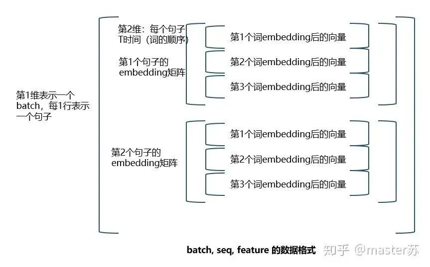
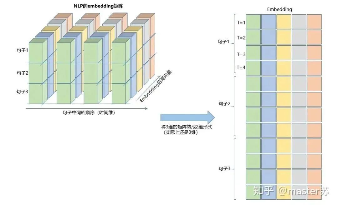
This just swaps the first two parameters. This is actually a relatively easy-to-understand data format. Below, I will illustrate how to construct the LSTM input using the embedding vector in NLP.Previously, our embedding matrix was as shown in the diagram below:If we place the batch first, the three-dimensional matrix format is as follows:The conversion process is shown in the diagram below:Did you understand? This is the format of the input data, isn’t it simple?The other two inputs for LSTM are h0 and c0, which can be understood as the network’s initialization parameters, which can be generated using random numbers.
h0(num_layers * num_directions, batch, hidden_size)
c0(num_layers * num_directions, batch, hidden_size)
Parameters include:
num_layers: number of hidden layers    num_directions: if it is a unidirectional recurrent network, then num_directions=1, if bidirectional then num_directions=2    batch: input data batch    hidden_size: number of hidden layer neurons
4.3 Output Format of LSTMThe output of LSTM is a tuple as follows:
output,(ht, ct) = net(input) output: output of the hidden layer neurons at the last state ht: state value of the hidden layer at the last state ct: forget gate value of the hidden layer at the last state
After saying so much, let’s look back at where ht and ct are, please see the diagram below:Where is the output? Please see the diagram below:LSTM Combined with Other NetworksDo you remember? The dimension of the output equals the number of hidden layer neurons, which is hidden_size. In some time series predictions, a fully connected layer is often added after the output, where the input dimension of the fully connected layer equals the LSTM’s hidden_size, and the subsequent network processing is the same as that of BP networks, as shown in the diagram below:Implementing the above structure in PyTorch:
import torch
from torch import nn
class RegLSTM(nn.Module):    def __init__(self):        super(RegLSTM, self).__init__()        # Define LSTM        self.rnn = nn.LSTM(input_size, hidden_size, hidden_num_layers)        # Define regression layer network, input feature dimension equals LSTM output, output dimension is 1        self.reg = nn.Sequential(            nn.Linear(hidden_size, 1)        )
    def forward(self, x):        x, (ht, ct) = self.rnn(x)        seq_len, batch_size, hidden_size = x.shape        x = y.view(-1, hidden_size)        x = self.reg(x)        x = x.view(seq_len, batch_size, -1)        return x
Of course, some models use the output as the input to another LSTM or use the information of the hidden layers ht, ct for modeling, and so on.Reference Links:https://zhuanlan.zhihu.com/p/94757947https://zhuanlan.zhihu.com/p/59862381https://zhuanlan.zhihu.com/p/36455374https://www.zhihu.com/question/41949741/answer/318771336https://blog.csdn.net/android_ruben/article/details/80206792
Download 1: OpenCV-Contrib Extension Module Chinese Version Tutorial
Reply with "OpenCV Extension Module Chinese Tutorial" in the background of the "Learn Visuals" WeChat public account to download the first Chinese version of the OpenCV extension module tutorial available online, covering installation of extension modules, SFM algorithms, stereo vision, target tracking, biological vision, super-resolution processing, and more than twenty chapters of content.

Download 2: 52 Lectures on Python Visual Practical Projects
Reply with "Python Visual Practical Projects" in the background of the "Learn Visuals" WeChat public account to download 31 visual practical projects including image segmentation, mask detection, lane line detection, vehicle counting, eyeliner addition, license plate recognition, character recognition, emotion detection, text content extraction, facial recognition, etc., to help quickly learn computer vision.

Download 3: 20 Lectures on OpenCV Practical Projects
Reply with "20 Lectures on OpenCV Practical Projects" in the background of the "Learn Visuals" WeChat public account to download 20 practical projects based on OpenCV, to achieve advanced learning of OpenCV.

Group Chat

Welcome to join the public account reader group to communicate with peers. Currently, there are WeChat groups for SLAM, 3D vision, sensors, autonomous driving, computational photography, detection, segmentation, recognition, medical imaging, GAN, algorithm competitions, etc. (will be gradually subdivided later). Please scan the WeChat ID below to join the group, and note: "Nickname + School/Company + Research Direction", for example: "Zhang San + Shanghai Jiao Tong University + Visual SLAM". Please follow the format, otherwise, it will not be approved. After successfully adding, you will be invited to relevant WeChat groups based on your research direction. Please do not send advertisements in the group, otherwise, you will be removed from the group. Thank you for your understanding.~