Click the above“Beginner Learning Vision“, choose to add “Starred” or “Pinned“
Important content delivered in real time
In deep learning, CNN networks are core components. For CNN networks, the calculations of convolutional layers and pooling layers are crucial. Different strides, padding methods, kernel sizes, and pooling strategies can significantly impact the final output model, parameters, and computational complexity. This article will start from the calculations of convolutional layers and pooling layers, demonstrating the differences in calculation results based on different strides, padding methods, and kernel sizes.
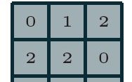
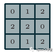
The Convolutional Neural Network (CNN) was first proposed in 1997 in a paper by Yann LeCun on digital OCR recognition. In the 2012 ImageNet competition, CNN networks successfully outperformed other non-DNN model algorithms, gaining attention from academia and interest from industry. Undoubtedly, to learn deep learning, one must learn about CNN networks, and to learn CNN, one must understand the foundational layers such as convolutional layers and pooling layers, as well as their parameter significance. Essentially, image convolution is discrete convolution, and image data is generally multi-dimensional (at least two dimensions). Discrete convolution is fundamentally a linear transformation with sparsity and parameter reuse characteristics, meaning the same parameters can be applied to different small blocks of the input image. Assuming we have a 3×3 discrete convolution kernel as follows:
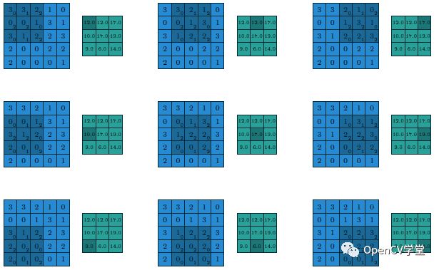
Assuming we have:
-
A 5×5 image input block
-
Stride of 1 (strides=1)
-
Padding method as VALID (Padding=VALID)
-
Kernel size (filter size=3×3)
Then their calculation process and output are as follows:
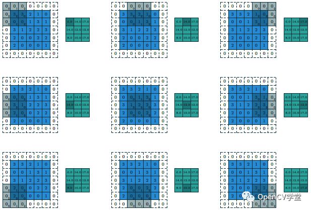
Now, if we change the stride to 2, padding method to SAME, and keep the kernel size unchanged (strides=2 Padding=SAME filter size=3×3), the calculation process and output change to:
The final output can be referred to as feature map. The depth of a CNN often refers to the number of feature maps. For multi-dimensional input images, calculating multiple convolution kernels results in multiple feature maps, which are then combined, as shown below:
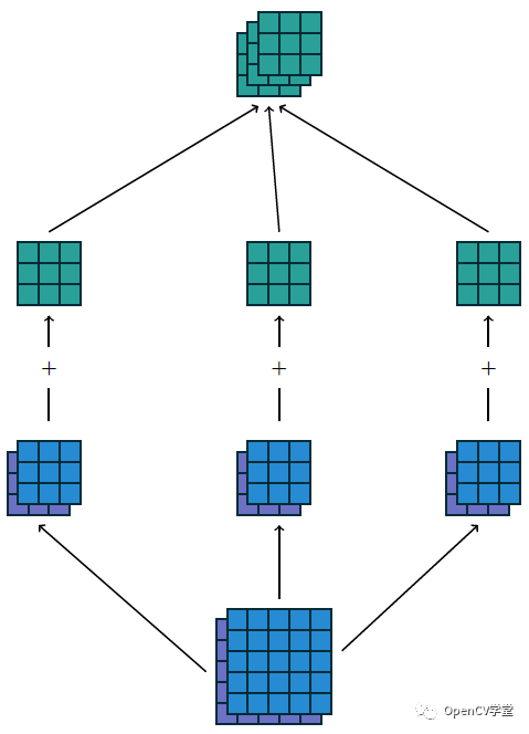
The above input is 5x5x2, using a 3×3 convolution kernel, resulting in 3x3x3 output, with VALID padding. If the padding method is changed to SAME, the output will be 5x5x3. This shows the impact of padding methods on output results.
In AlexNet, there are 11×11 and 5×5 convolution kernels, but in VGG networks, due to the increased number of layers, the convolution kernels have changed to sizes 3×3 and 1×1. This has the advantage of reducing the computational load during training, which helps lower the total number of parameters. There are essentially two methods to replace large convolution kernels with small ones.
1. Decomposing 2D Convolution into Two Continuous 1D Convolutions
2D convolutions can be decomposed into two 1D convolutions, which is mathematically justified. Therefore, an 11×11 convolution can be transformed into two consecutive convolutions with kernels 1×11 and 11×1. The total number of operations is:
11x11 = 121 times
1x11 + 11x1 = 22 times
2. Replacing Large 2D Convolutions with Multiple Continuous Small 2D Convolutions
It can be seen that changing a large 2D convolution kernel in the computation process to two consecutive small convolution kernels can greatly reduce the number of calculations and computational complexity. Similarly, a large 2D convolution kernel can also be replaced by several small 2D convolution kernels. For example, for a 5×5 convolution, we can replace it with two consecutive 3×3 convolutions, comparing the number of operations:
5x5 = 25 times
3x3 + 3x3 = 18 times
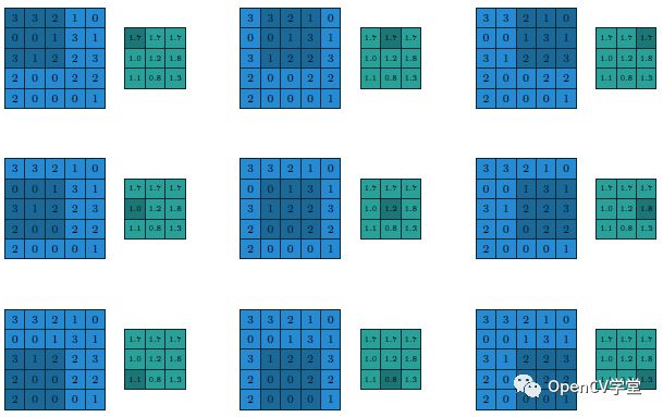
In CNN networks, a pooling layer follows the convolutional layer. The role of the pooling layer is to extract local means and maximum values. Depending on the calculated values, it can be divided into average pooling layers and max pooling layers, with max pooling layers being the most common. During pooling, it is also necessary to provide the filter size and stride. Below is the average pooling calculation process and output results of a 3×3 filter with a stride of 1 on a 5×5 input image:
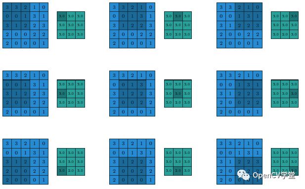
The process and results of using max pooling are as follows:
Discussion Group
Welcome to join the reader group of the official account to exchange ideas with peers. Currently, we have WeChat groups for SLAM, 3D Vision, Sensors, Autonomous Driving, Computational Photography, Detection, Segmentation, Recognition, Medical Imaging, GAN, Algorithm Competitions, etc. (these will be gradually subdivided). Please scan the WeChat ID below to join the group, and note: “Nickname + School/Company + Research Direction”, for example: “Zhang San + Shanghai Jiao Tong University + Vision SLAM”. Please follow the format; otherwise, you will not be approved. After successful addition, you will be invited to enter the relevant WeChat group based on your research direction. Please do not send advertisements in the group, otherwise, you will be removed from the group. Thank you for your understanding~