Deep Learning LSTM for Stock Trading: Hedge Fund Case Study

Big Data Digest Work

Compiled by: Wang Yiding, Xiu Zhu, Ruan Xuenni,Ding Hui, Qian Tianpei

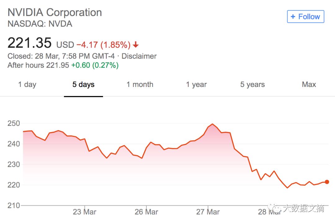
NVIDIA released the “world’s largest GPU” yesterday while experiencing a stock price drop of more than $20, which has not recovered by the time of this publication. Countless students are asking in the background whether they should buy the dip?

Today, using deep learning sequence models to predict stock prices has achieved good results, especially in hedge funds. Stock price data is a typical time series data.

What is sequence data? Data such as speech and text that have a temporal correlation and order can be regarded as sequence data.

Applying sequence models to speech and text, deep learning has achieved astonishing results in tasks such as speech recognition, reading comprehension, and machine translation.

How to operate specifically? What are the effects? Let’s take a look at this deep learning stock trading guide brought to you by the Digest.

Hedge funds are one of the attractive fields for the application of deep learning and a form of investment fund. Many financial organizations raise funds from investors and manage them, making predictions by analyzing time series data. In deep learning, a suitable architecture for time series analysis is: Recurrent Neural Networks (RNNs), more specifically, a special type of RNN: Long Short-Term Memory networks (LSTMs).

RNNs Wikipedia explanation:

https://en.wikipedia.org/wiki/Recurrent_neural_network

LSTM Wikipedia explanation:

https://en.wikipedia.org/wiki/Long_short-term_memory

LSTMs can capture the most important features from time series data and perform associative modeling. Stock price prediction models are a typical case of how hedge funds use such systems, trained using the PyTorch framework written in Python, designed experiments and plotted results.

Before introducing real cases, let’s first understand the basics of deep learning:

• First, introduce the abstract concept of deep learning.

• Secondly, introduce RNNs (or more specifically LSTMs) and how they perform time series analysis.

• Next, familiarize the readers with financial data suitable for deep learning models.

• Then, give an example to illustrate how a hedge fund uses deep learning to predict stock prices.

• Finally, provide actionable advice on how to use deep learning to improve the performance of existing or newly purchased hedge funds.

Introduction to a Case of Trading Using Deep Learning

One of the most challenging and exciting tasks in the financial industry is: predicting whether future stock prices will go up or down. As far as we know, deep learning algorithms are very good at solving complex tasks, so it is worth trying whether deep learning systems can successfully solve the problem of predicting future prices.

Stock price prediction:

https://www.toptal.com/machine-learning/s-p-500-automated-trading

The concept of artificial neural networks has existed for a long time, but due to hardware limitations, rapid experimentation in deep learning has not been possible. Ten years ago, NVIDIA developed high-speed computing graphics processing units (GPUs) for its Tesla series products, which facilitated the development of deep learning networks. In addition to providing higher quality graphics display in gaming and professional design programs, highly parallelized GPUs can also compute other data, and in many cases, they outperform CPUs.

NVIDIA Tesla Wikipedia explanation:

https://en.wikipedia.org/wiki/Nvidia_Tesla

There are not many scientific papers applying deep learning in the financial field, but financial companies have a great demand for deep learning experts, clearly recognizing the application prospects of deep learning.

This article will attempt to illustrate: why deep learning is becoming increasingly popular in building deep learning systems with financial data, and also introduce LSTMs, a special type of recurrent neural network. We will outline how to use recurrent neural networks to solve finance-related problems.

This article also provides a typical case analysis of how hedge funds use deep learning systems, showcasing the experimental process and results. At the same time, we will analyze how to improve the performance of deep learning systems and how to build deep learning systems for hedge funds by bringing in talent (what kind of background deep learning talent is needed).

What Makes Hedge Funds Different

Before we delve into the technical aspects of this issue, we need to explain what makes hedge funds different. First, what is a hedge fund?

A hedge fund is a type of investment fund where financial organizations raise funds from investors and invest them in short-term and long-term investment projects or different financial products. Its form is generally a limited partnership or a limited liability company.

The goal of a hedge fund is to maximize returns, which are the gains or losses of its net worth over a specific period. It is generally believed that the greater the investment risk, the greater the corresponding return or loss.

To achieve good returns, hedge funds rely on various investment strategies, trying to make money by exploiting market inefficiencies. Because hedge funds have various investment strategies not allowed for ordinary investment funds, they are not recognized as general funds and are not regulated by the state like other funds.

Therefore, they do not need to disclose their investment strategies and business results, which may make related operations full of risks. While some hedge funds generate returns above the market average, others have lost funds. Some of these losses are irretrievable, and some hedge funds’ results are reversible.

By investing in hedge funds, investors can increase the net worth of the fund. However, not everyone can invest in hedge funds; they are only suitable for a few wealthy investors. Generally, those who want to participate in hedge fund investments need to obtain certification.

This means they must have a special status in financial regulatory law. Different countries have different definitions of “special status.” Typically, an investor’s net worth needs to be very high—not just for individuals, but banks and large companies can also operate in hedge funds. This certification is designed to ensure that only individuals with necessary investment knowledge can participate, thus protecting inexperienced small investors from risks.

The United States is the most developed country in the global financial market; therefore, this article mainly references the U.S. regulatory system. In the United States, the Securities and Exchange Commission (SEC) Rule D 501 defines the term “accredited investor.”

According to this regulation, an accredited investor can be:

• Banks

• Private enterprises

• Organizations

• Directors, executives, and general partners of the issuing organizations providing or selling securities

• Individuals with a net worth exceeding $1,000,000, either individually or jointly with their spouse

• Individuals with an annual income exceeding $200,000 in each of the last two years, or a joint income with their spouse exceeding $300,000, and the expected income for the current year also reaching the same level.

• Trusts with total assets exceeding $5,000,000

• Entities where all equity owners are accredited investors

Hedge fund managers must find a way to create a competitive advantage to succeed, that is, to be more creative and bring greater value than competitors. This is a very attractive career choice because if a person is good at managing funds, they can profit significantly.

On the other hand, if many hedge fund managers make poor decisions, they will not only fail to earn profits but may also cause negative effects. The best hedge fund managers can earn the highest-paying positions in the industry.

In addition to management fees, hedge fund managers can also take a cut from the profits. This compensation method encourages hedge fund managers to invest more aggressively for higher returns, but at the same time, it also exposes investors to more risks.

A Brief History of Hedge Funds

The first hedge fund appeared in 1949, founded by writer and sociologist Alfred Winslow Jones. In 1948, Alfred published an article on the investment trends at the time.

He achieved great success in fund management. By using his investment innovations to raise funds, this investment innovation is now widely known as long/short equity. This strategy remains very popular in hedge funds today. Stocks can be bought (long) or sold (short).

When stock prices are low but expected to rise, one buys the stock (long), and once it reaches a high price, they sell (short). This is the core of Alfred’s theory—holding long positions in stocks expected to appreciate and short positions in stocks expected to decline.

Financial Data and Datasets

Financial data belongs to time series data. Time series is a series of data points ordered in time. Typically, time series is continuous, equidistant time series: that is, discrete time series data. For example, the height of ocean tides, the number of sunspots, and the daily closing price of the Dow Jones Industrial Average are all time series.

The historical data here refers to past time series data. This is the most important and valuable part for predicting future price trends.

There are some publicly available datasets online, but usually, the data lacks many features—such as data at 1-day intervals, 1-hour intervals, or 1-minute intervals.

Datasets with richer features and smaller time intervals are usually not publicly available and need to be purchased at a high price.

Smaller intervals mean more time series data in a fixed period—there are 365 (or 366) days in a year, so there can be up to 365 (or 366) data points available. There are 24 hours in a day, so there are 8,760 (or 8,784) hourly data points in a year, and there are 525,600 (or 527,040) minute data points in a year.

More data means more available information, which also means better judgment of what will happen next—of course, if the data contains enough features, it can generalize well.

During the peak of the global financial crisis, stock price data from 2007 to 2008 may not predict recent price trends due to biases. Smaller time intervals result in more data points within a fixed period, making it easier to predict what will happen next.

If we have data for every nanosecond over n years, it will be easy to predict what will happen in the next nanosecond. Similarly, in the stock market, having data over a certain period makes it much easier to predict what will happen next.

Of course, this does not mean that only short-term predictions made after a series of data are correct; long-term predictions can also be correct.

Each short-term prediction will produce errors, so linking multiple predictions will ultimately produce larger errors in long-term predictions, rendering them invalid. Below is an example of Google stock data with a 1-day interval provided by Yahoo Finance.

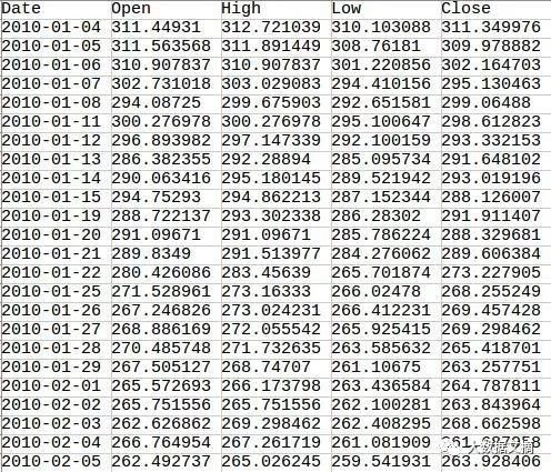
The dataset contains only five columns of data: date, opening price, highest price, lowest price, and closing price, which indicate the price at which the security first trades when the market opens, the highest price reached on that trading day, the lowest price on that trading day, and the final price of the traded security on that day.

Usually, such datasets also have two columns—”adjusted closing price” and “volume,” but they are not relevant here. The adjusted closing price refers to the closing price after adjustments for splits and dividend distributions, while volume refers to the number of stocks traded in the market over a given period.

It can be seen that some dates are missing in the data. These are the days when the stock exchange is closed (usually on weekends and holidays).

To demonstrate the deep learning algorithm, the closed prices for closed days use the previous trading day’s prices. For example, on 2010-01-16, 2010-01-17, and 2010-01-18, the closing price will all be 288.126007 because that is the price from 2010-01-15. For our algorithm, it is essential that the data has no gaps, so we will not confuse it.

The deep learning algorithm can learn from data over weekends and holidays— for instance, learning that there will be two days of flat prices after the last working day over five working days.

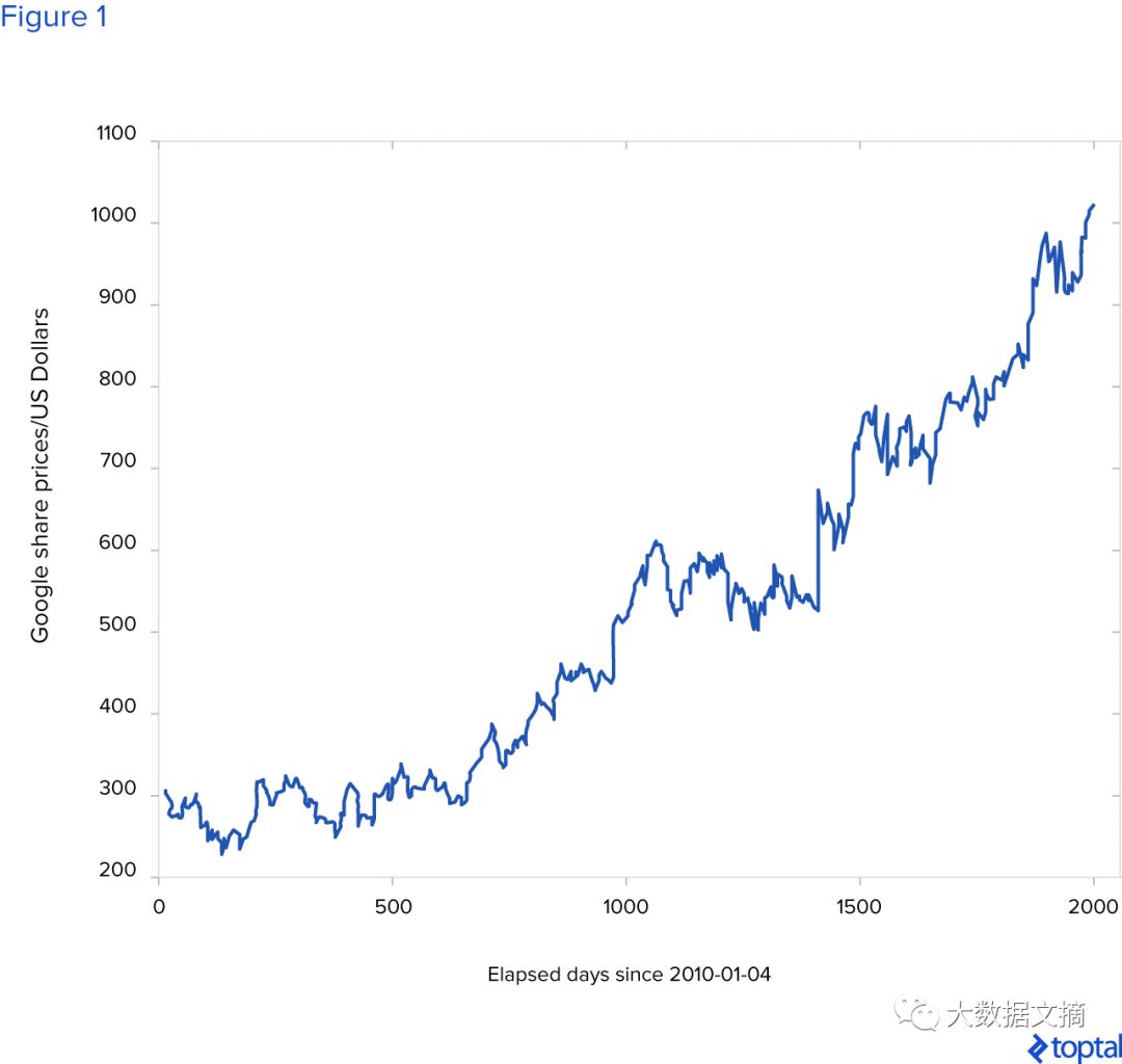
This is a chart showing the fluctuations of Google’s stock price since 2010-01-04. Note that the chart only shows changes on trading days.

What is Deep Learning?

Deep learning is based on data representation learning and is a branch of machine learning. Machine learning is not programmed but learned from data algorithms. It is essentially a method of artificial intelligence.

Deep learning has been applied in various fields: computer vision, speech recognition, natural language processing, machine translation, and in some tasks, its performance even surpasses that of humans.

Deep Neural Networks are at the core of deep learning, and the simplest, most basic example is the feedforward neural network. As shown in the figure below, a basic feedforward neural network includes an input layer, an output layer, and hidden layers.

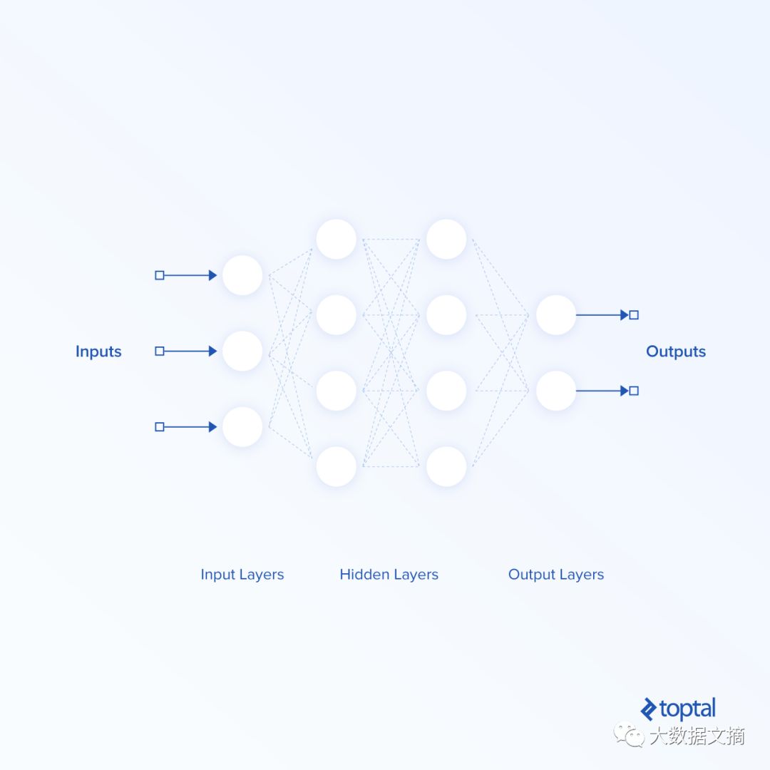
The hidden layers are multiple individual layers between the input and output layers. We generally say that if a neural network has more than one hidden layer, then the network is deep.

Each layer consists of a different number of neurons. The layers in this basic feedforward neural network are called linear layers, where neurons simply multiply the 1-D (or 2-D, if the data is batched) input by the appropriate weights and sum them to yield the final result as a 1-D or 2-D output.

Activation functions are usually introduced in feedforward networks to represent nonlinear relationships, thereby modeling more complex nonlinear problems. In a feedforward neural network, data flows from the input layer to the output layer and does not backpropagate.

The connections between neurons are weighted. These weights need to be adjusted so that the neural network returns accurate outputs for given inputs. Feedforward networks map data from input space to output space. Hidden layers extract important and more abstract features from the previous layer’s features.

The general deep learning pipeline, like the machine learning pipeline, includes the following steps:

1. Data collection. The data is divided into three parts: training set, validation set, and test set.

2. Using the training set to train the DNN model for multiple rounds (each round includes multiple iterations), and validating using the validation set after each round of training.

3. After continuous training and validation, testing the model (an instance of the neural network with fixed parameters).

Training the neural network is essentially about minimizing the loss function by combining the backpropagation algorithm with stochastic gradient descent to continuously adjust the weights between neurons.

In addition to the weights determined through the learning process, deep learning algorithms usually also require the setting of hyperparameters—parameters that cannot be obtained from the learning process but need to be determined before the learning process. Parameters such as the number of network layers, the number of neurons in the network layers, the types of network layers, the types of neurons, and initial weights are all considered hyperparameters.

In hyperparameter settings, the first limitation is hardware; currently, it is impossible to set a trillion neurons on a single GPU. The second hyperparameter search problem belongs to combinatorial explosion; thoroughly searching all possible combinations of hyperparameters is impossible, as this process would take infinitely long.

For these reasons, hyperparameter settings are usually random or use some heuristic methods and some well-known methods provided in the literature—this article will later show an example of hyperparameter settings for recurrent neural networks used in financial data analysis, which many scientists and engineers have proven to perform well in processing time series data.

Generally, the best way to validate whether a hyperparameter is effective for a specified problem is to conduct experiments.

The purpose of training is to ensure that the neural network fits the training data well. Validation after each training step and testing the model after the entire training process are designed to determine whether the model has good generalization ability.

Strong generalization ability means that the neural network model can make accurate predictions for new data.

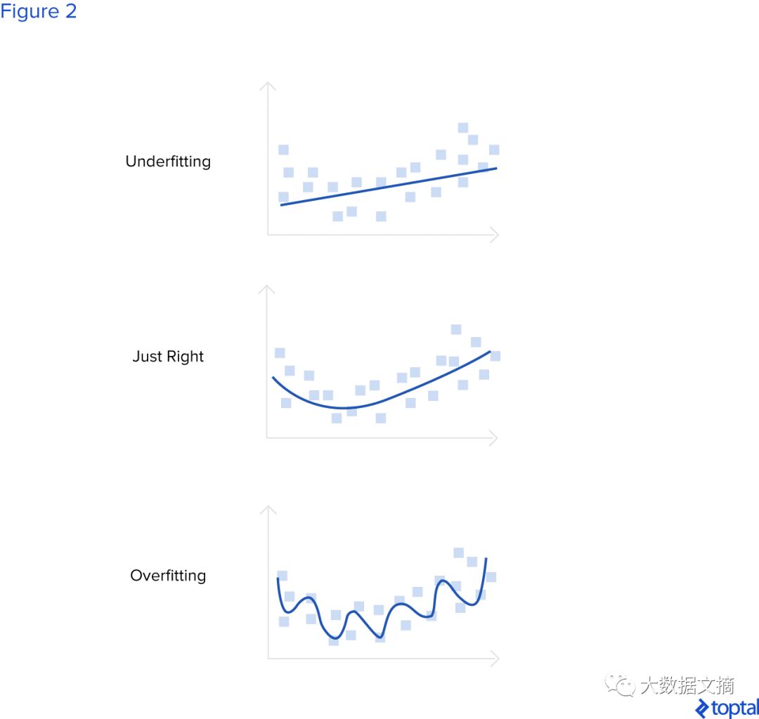
There are two important terms regarding model selection: overfitting and underfitting. If a neural network is too complex for the data it was trained on—if it has too many parameters (too many layers and/or too many neurons in the layers)—then this neural network is likely to overfit.

Because it has enough capacity to fit all the data, it can adapt well to the training data, but this model will perform poorly on the validation and test sets. If a neural network is too simple for the data it was trained on, this model will underfit.

In this case, the neural network performs poorly on the training set, validation set, and test set because it lacks the capacity to fit the training data and generalize. In the following figure, we explain these terms graphically.

The blue line represents the neural network model. The first figure shows the situation where the neural network cannot fit the training data and generalize when the parameters of the neural network are few. The second figure shows that when there is an optimal number of parameters, the neural network has good generalization ability to new data. The third figure shows that when the neural network has too many parameters, this model overfits the training data but performs poorly on the validation and test sets.

Recurrent Neural Networks

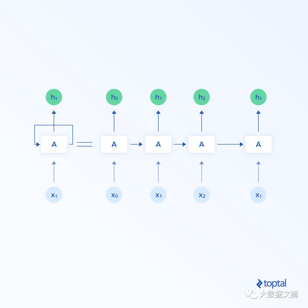
A more complex version in neural networks is the Recurrent Neural Network (RNN). Unlike feedforward neural networks, data in RNNs can flow in any direction. RNNs can better represent the correlations in time series. The general structure of RNNs is shown in the figure below.

A recurrent neuron is represented as shown in the figure below. At time t, inputting X_{t} returns the hidden state h_{t} as output, and the hidden layer output backpropagates to the neuron. The representation of the recurrent neuron when unfolded is shown in the right part of the figure. X_{t_0} represents the point at time t_{0}, X_{t_1} represents the point at time t_{1}, and X_{t} represents the point at time t. The outputs obtained from inputs X_{t_0}, X_{t_1}, …, X_{t_n} at times t_{0}, t_{1}, …, t_{n} are called hidden outputs, i.e., h_{t_0}, h_{t_1}, …, h_{t_n}.

The most effective RNN architecture is the LSTM structure. It is represented as follows:

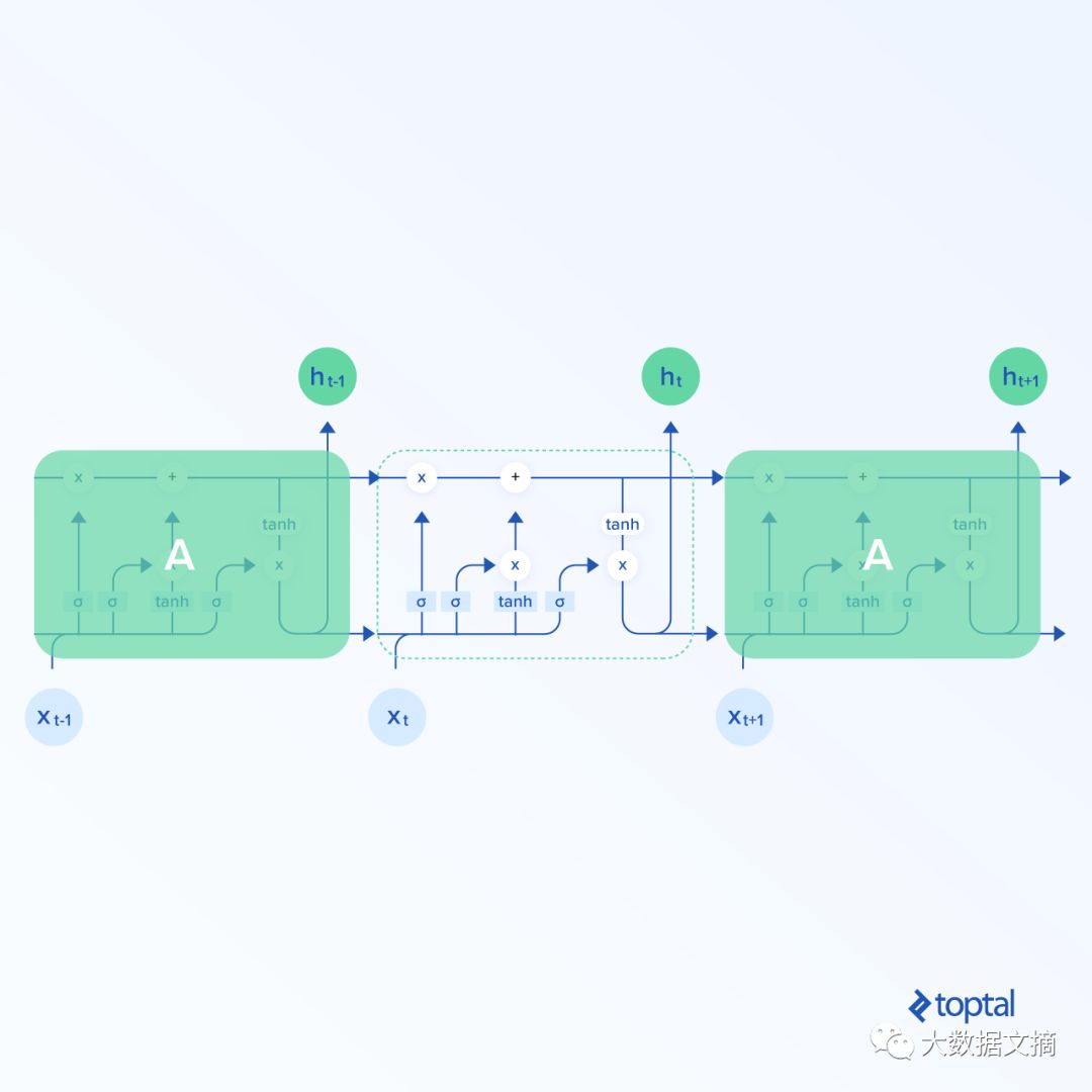
LSTMs have a structure similar to general RNNs, but the structure of the recurrent neurons is more complex. As can be seen from the figure above, there are many computations within an LSTM unit.

In this article, the LSTM unit can be viewed as a black box, but for curious readers, there is a blog that explains the computations within LSTMs and some other content.

Blog link:

http://colah.github.io/posts/2015-08-Understanding-LSTMs/

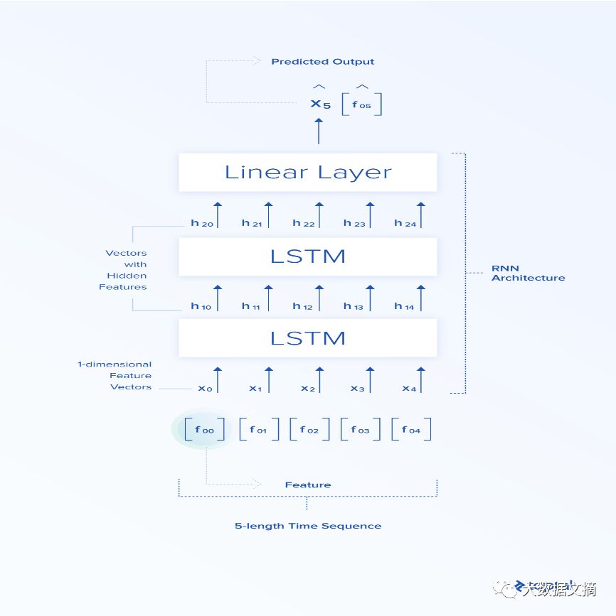
We refer to the input of the neural network as the “feature vector.” This is an n-dimensional vector whose elements are features: f_{0}, f_{1}, f_{2}, …, f_{n}. Now, let’s explain how recurrent neural networks are applied to finance-related tasks. The input to the RNN is [X_{t_0}, X_{t_1}, X_{t_2}, …, X_{t_n}]. Here we let n=5.

We use Google’s stock closing prices over five consecutive days (see the opening/high/low/closing data table above) from 2010-01-04 to 2010-01-08, i.e., [[311.35], [309.98], [302.16], [295.13], [299.06]]. The feature vector in this example is one-dimensional. The time series consists of five such feature vectors. The output of the RNN is the hidden features [h_{t_0}, h_{t_1}, h_{t_2}, …, h_{t_n}].

These features are more abstract than the input features [X_{t_0}, X_{t_1}, X_{t_2}, …, X_{t_n}], as LSTM needs to learn the important parts of the input features and map them to the hidden feature space.

These hidden abstract features propagate in the next LSTM unit and provide a set of hidden, more abstract features that can propagate in the next LSTM unit, and so on.

After connecting sequences in LSTMs, the last component of the neural network is the linear layer (the part of the simple feedforward network introduced in the previous section), which maps the final LSTM hidden vector to a point in one-dimensional space, which is the final output of the network—the predicted closing price in time period X_{t+1}. In this example, it should be 298.61.

Note: There are also a small number of LSTMs that take the number of LSTMs as a hyperparameter, which is usually obtained through experience, but can also use some heuristic methods. If the data is not very complex, we can use a less complex structure to avoid overfitting. If the data is more complex, we use a more complex model to prevent underfitting.

During the training process, the predicted closing price will be compared with the actual price, and the difference will be minimized using the backpropagation algorithm and gradient descent optimization algorithm (or other forms—specifically, in this article, the “Adam” version of the gradient descent optimization algorithm will be used) by changing the weights of the neural network.

Once the model is trained and tested, in future use, the user only needs to input data into the model, and the model will return the predicted value (ideally, the price will be very close to the actual future price).

One more thing to note is that generally, in the training and testing part, data is passed through the network in batches, allowing the network to compute multiple outputs in one go.

The figure below shows the architecture used in this article, including 2 LSTM stacks and a linear layer.

Hedge Fund Algorithm Experiment

Try to implement an algorithm with a simple trading strategy, described as follows: If the algorithm predicts that the stock price will rise tomorrow, buy n (in this example, n=1 share of the company’s stock (long), otherwise sell all the stocks of the company held (short).

The initial value of the portfolio (the total value of cash and stocks) is set at $100,000. Each trading action will buy n shares of the company (taking Google as an example) or sell all the stocks held of the company. At the initial moment, the system holds 0 shares of the given company’s stock.

It is essential to remember that this is a very basic and simple example, not suitable for real life. If you want this model to be well applied in practice, much R&D work is still needed to adjust the model.

Some factors ignored in this example should be considered in practical scenarios: for instance, trading costs are not accounted for in the model. Moreover, it is assumed that the system can trade at the same time every day and treats every day, even weekends or holidays, as a trading day.

For model testing, we use the backtesting method. This method uses historical data to recreate trades that should have occurred based on the rules defined by the developed strategy. We divide the dataset into two parts—the first part as the training set (as historical trading data), and the second part as the test set (as future trading data).

The model is trained on the training set, and after training is complete, we predict future trades on the second test set to verify the performance of the trained model on “future trading” data that does not belong to the training set.

The metric used to evaluate the trading strategy is the Sharpe ratio (annualized, assuming every day of the year is a trading day, with 365 days: sqrt(365)*mean(returns)/std(returns)), where the return is defined as p_{t}/p_{t-1} – 1, with p_{t} being the price at time t.

The Sharpe ratio reflects the ratio of the portfolio’s return to the additional risk, so the larger the Sharpe ratio, the better. Generally, for investors, a Sharpe ratio greater than 1 is satisfactory, greater than 2 is very good, and greater than 3 is excellent.

In this example, we only used the daily closing prices of Google’s historical prices from Yahoo Finance dataset as features. While other features are also useful, discussing whether other features in this dataset (opening price, highest price, lowest price) are effective is not within the scope of this article.

Other features not included in this data table may also be useful—for example, news sentiment at a specific minute or significant events that occurred on a particular day.

However, it is sometimes challenging to represent these features as useful inputs for neural networks and combine them with existing features. For instance, for each given period, it is easy to expand the feature vector and add a representation of news sentiment or Trump’s sentiment in a tweet (where -1 indicates agreement, 0 indicates neutral, and +1 indicates disagreement).

However, adding specific event-driven moments (such as the piracy incident in the Suez Canal or the discovery of a bomb at a Texas refinery) to the feature vector is not easy, because for each such specific moment, we need to add an extra element to the feature vector that becomes 1 when the event occurs and 0 otherwise.

Thus, to consider all possible specific moments, we need to add infinitely many elements to the feature vector.

For more complex data, we can define categories for each specific moment to determine which category it belongs to. We can also add features from other companies’ stock prices to let the model learn the correlations between the stock prices of different companies.

Additionally, we can combine recurrent layers with another type of neural network specialized for computer vision—convolutional neural networks—to explore how visual features are associated with certain companies’ stock prices, which is also an interesting approach.

Perhaps we can use a photo of a crowded train station taken with a camera as a feature and add it to the neural network to explore whether what the neural network “sees” is related to the stock prices of certain companies—perhaps there are hidden messages even in this mundane and absurd example.

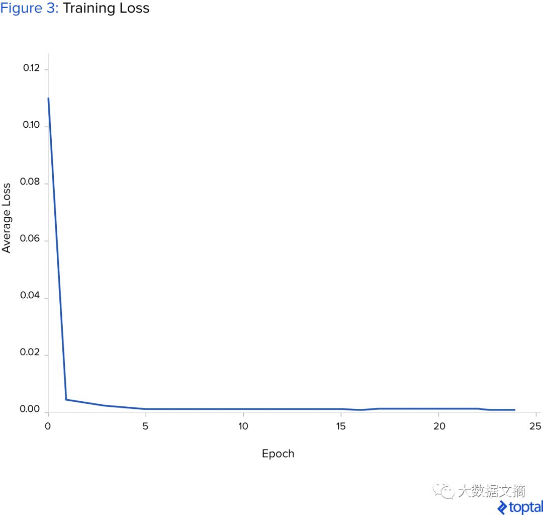
The figure below shows the process of average training loss decreasing over time, indicating that the neural network has enough capacity to fit the training set. It must be emphasized that data standardization is necessary to ensure that deep learning algorithms can converge.

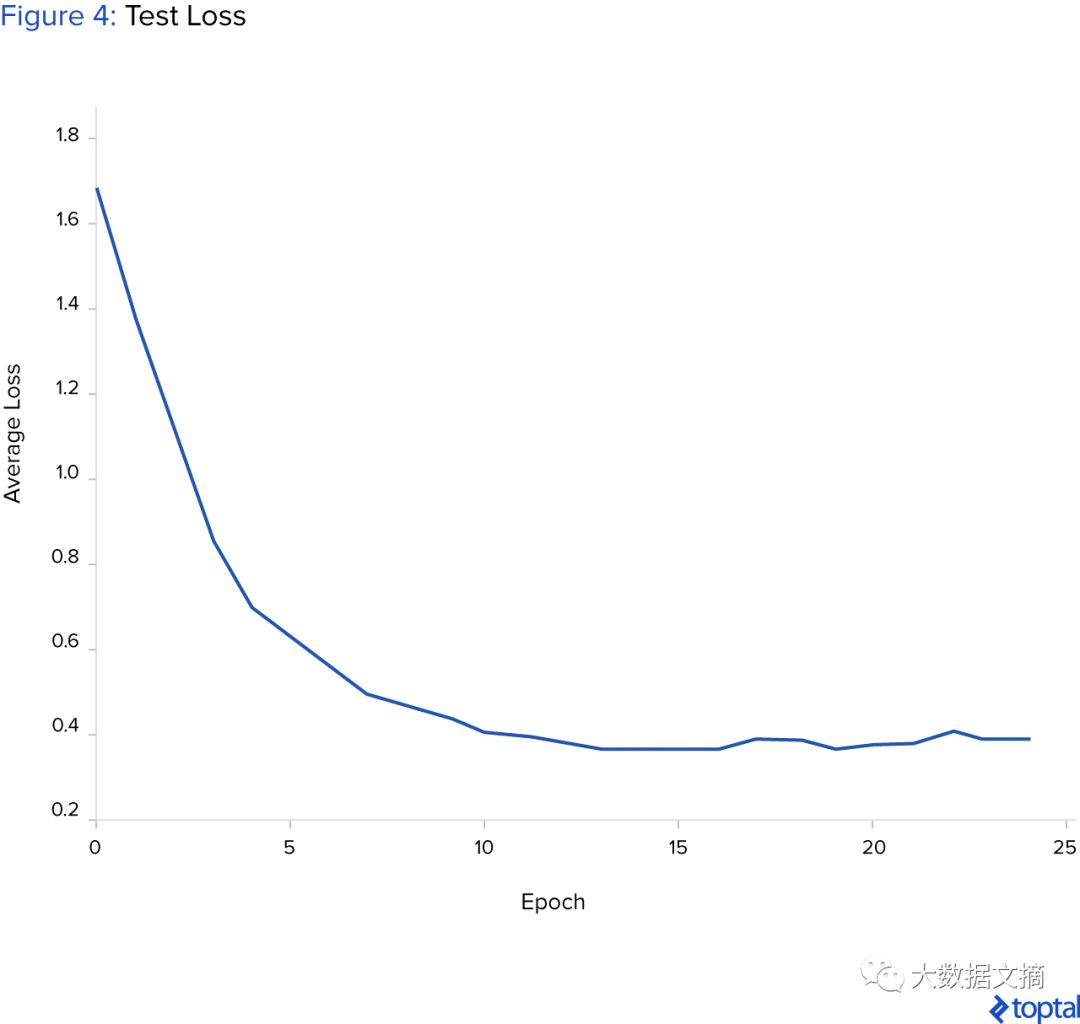
The figure below shows the process of average test loss decreasing over time, indicating that the neural network has some generalization ability for new data.

The algorithm has a greedy nature: If it predicts that tomorrow’s stock price will rise, the algorithm will immediately buy n=1 share of that company’s stock (if there is enough cash in the portfolio); otherwise, it will sell all stocks of that company held (if any).

The investment time period is fixed at 300 days. After 300 days, sell all stocks. The simulated results of the trained model on new data are shown in the figure below. The figure shows the changes in the portfolio’s value over time as trades are made long/short (or no trades).

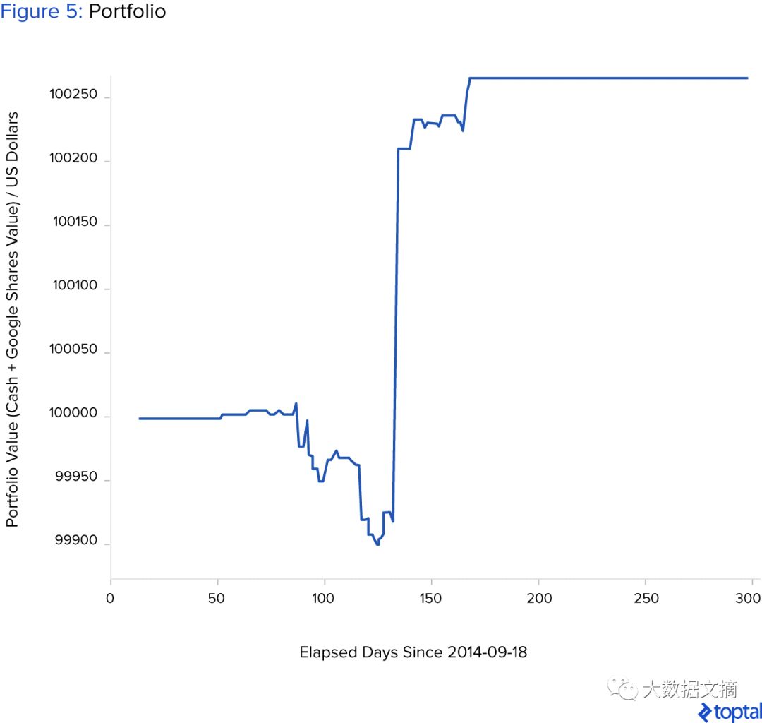
The Sharpe ratio of the above investment simulation is 1.48. The final value of the portfolio after 300 days is $100,263.79. If we only bought stocks on the first day and sold them after 300 days, the portfolio value would be $99,988.41.

The figure below shows the situation of losses after 300 days of fixed investment period due to poor training of the neural network.

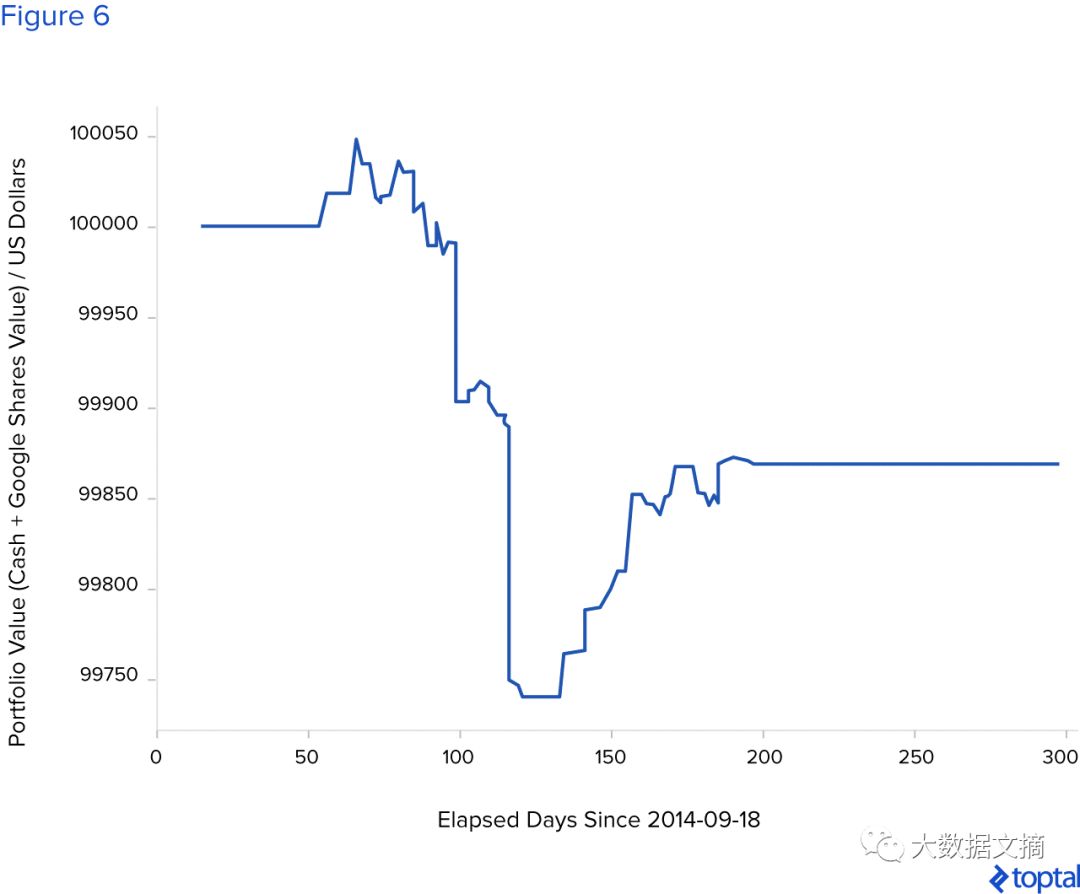
The Sharpe ratio of this simulation is -0.94. The final value of the portfolio after 300 days is $99,868.36.

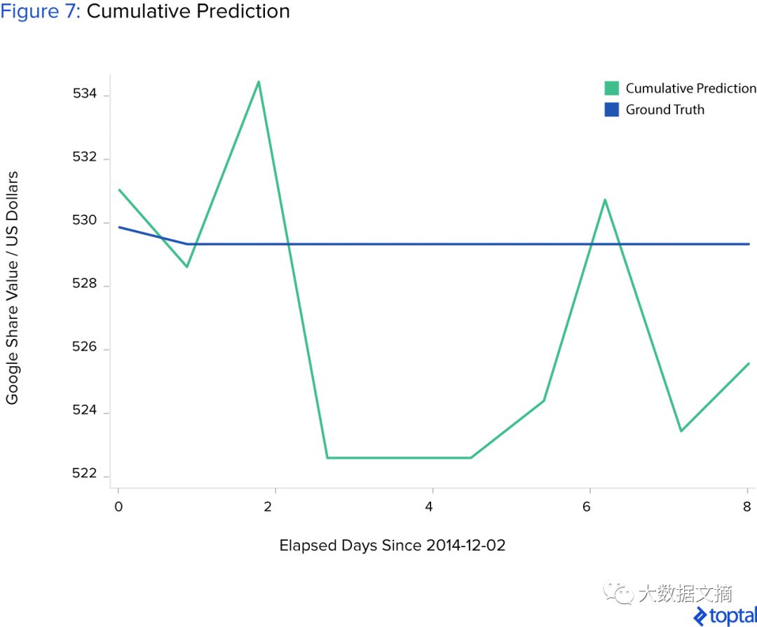
Here’s an interesting example: the above algorithm has a greedy nature and only estimates the stock price for the next day, making decisions based solely on this predicted value. However, it may still be necessary to connect multiple predicted values and forecast prices for multiple future periods.

For instance, with the first group of inputs [X_ground_truth_{t0}, X_ground_truth_{t1}, X_ground_truth_{t2}, X_ground_truth_{t3}, X_ground_truth_{t4}] and the first output [X_ground_truth_{t5}], we can input this predicted value into the neural network to continue predicting, i.e., the next group of inputs is [X_ground_truth_{t1}, X_ground_truth_{t2}, X_ground_truth_{t3}, X_ground_truth_{t4}, X_ground_truth_{t5}], and the output is [X_predicted_{t6}].

Similarly, the next group of inputs would be X_ground_truth_{t2}, X_ground_truth_{t3}, X_ground_truth_{t4}, X_predicted_{t5}, X_predicted_{t6}], which would yield [X_predicted_{t7}], and so on.

The problem here is that we introduce a prediction error, and this error increases with each new prediction step, ultimately leading to a very poor long-term prediction result, as shown in the figure below. Initially, the model’s predicted values have the same downward trend as the true values, but then stagnate and become worse over time.

A simple deep learning analysis of Google’s stock price shows that as long as the data volume is large enough and the quality is good enough, this model can almost encompass any financial dataset. However, the data must be discernible and well-represent the and describe the problem.

Conclusion

If the model performs well on a large number of tests and has strong generalization ability, then it can enable hedge fund managers to use deep learning and algorithmic trading strategies to predict the stock prices of future companies.

Hedge fund managers can input the amount of funds into the system to automate trading every day. However, allowing the automated trading algorithm to trade completely unsupervised is definitely not a good choice.

Therefore, hedge fund managers should have some knowledge of deep learning or hire someone with the necessary deep learning skills to supervise and judge whether this system has lost its generalization ability and is no longer suitable for trading.

Once the system loses its generalization ability, it is necessary to retrain the model from scratch and retest it (which can be done by introducing more discernible features or new information—using new historical data not used in the last training).

Sometimes, poor data quality can lead to the deep learning model not being well trained and generalized. In such cases, an experienced deep learning engineer should be able to identify and reverse this situation.

To build a deep learning trading system, you need hedge fund data scientists, machine learning/deep learning experts (including scientists and engineers), and R&D engineers familiar with machine learning/deep learning, etc.

No matter which field of application they are familiar with in machine learning, whether it is computer vision or speech recognition, seasoned experts should be able to apply their experience well in the financial field.

Ultimately, regardless of the application or industry, deep learning has the same foundation, so it should be simple for experienced individuals to switch from one topic to another.

The system described here is the most basic, and to apply it to the real world, more R&D work is needed to increase returns. Possible system improvement methods include developing better trading strategies.

Collecting more data to train the model is also helpful, but such data is generally expensive.

Shortening the intervals between time points can also improve the model. Using more features (such as news sentiment or significant events corresponding to each time point in the dataset, although it is challenging to represent them in a form suitable for neural networks), extensive grid search optimization of hyperparameters, and exploration of recurrent neural network structures can also enhance the model.

Additionally, when conducting numerous parallel experiments and processing large amounts of data (if a significant amount of data is collected), we also need more computing power (stronger GPUs are essential).

Original link:

https://www.toptal.com/deep-learning/deep-learning-trading-hedge-funds

[Today’s Machine Learning Concept]

Have a Great Definition

Countdown to Class: 3 Days

Data Science Bootcamp Session 5

Excellent Teaching Assistant Recommendation | Potato

In today’s chaotic data science training market, have you been dazzled and at a loss, still not found an organization? Don’t panic, the Potato veteran will hold your hand and earnestly guide you: what exactly is quality data science education and training?

The course is full of practical content while being engaging, the instructors are energetic and love to share, and the teaching assistants are diligent in grading and enthusiastic in feedback.

That’s right! The Data Science Bootcamp is such a star course! From basic Python programming and Scrapy crawling to proficient use of various Python libraries like Numpy/Pandas/Matplotlib/Seaborn/Scikit-learn, it covers the essentials of machine learning, transforming from a data science novice to an advanced player through real data science competition cases and data mining projects!

As a teaching assistant for sessions 4 and 5, I advise novice students: keep up with the course pace, complete all assignments on time, take good study notes, and you will surely achieve an easy entry into data science!

Volunteer Introduction