

Source: Machine Heart (ID: almosthuman2014)
[Introduction] Generative Adversarial Networks (GAN) can now synthesize highly realistic images, but a study by MIT, IBM, and the Chinese University of Hong Kong shows that GANs can miss certain details in the target distribution during image synthesis. Future GAN designers who can fully consider these omissions should be able to create higher quality image generators. The researchers have released related papers, code, and data.
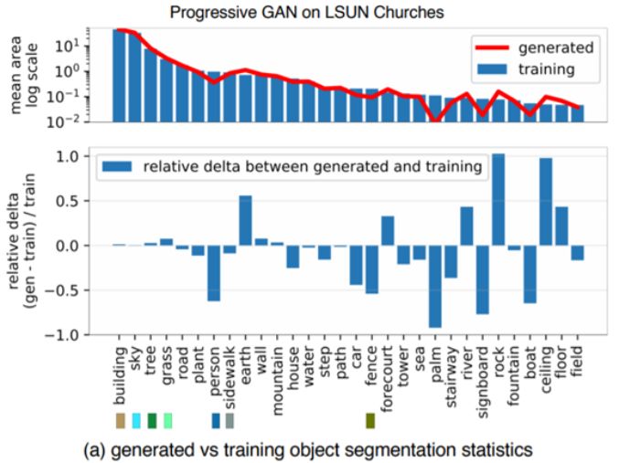
First, the authors deployed a semantic segmentation network to compare the generated images with the segmented target distribution in the training set. The statistical differences can reveal the target categories ignored by the GAN.
Figure 1a shows that in a church GAN model, categories such as people, cars, and fences appear with fewer pixels in the generated distribution compared to the training distribution.
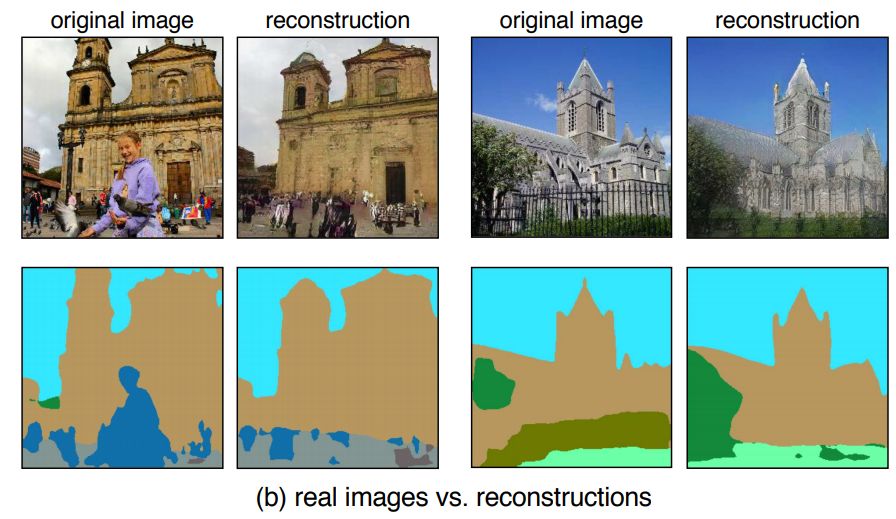
Then, given the identified omitted target categories, the authors directly visualized the omissions of the GAN. Specifically, the authors compared the specific differences between each photo and the images closely generated by the GAN. To do this, the authors relaxed the constraints of the inverse problem and solved an easier inverse problem of one layer of the GAN (rather than the entire generator).
In the experiments, the authors applied this framework to analyze several recent GANs trained on different scene datasets. The authors were surprised to find that the missing target categories did not appear distorted, poorly rendered, or rendered as noise. On the contrary, they were completely omitted, as if the object was not part of the scene at all. Figure 1b provides an example, showing that a larger person was completely skipped, and the parallel lines of the fence were completely ignored. Thus, GANs may ignore categories that are too difficult to handle while still achieving higher average visual quality outputs. For related code, data, and other information, see: ganseeing.csail.mit.edu.
Quantifying Mode Collapse at the Distribution Level
The systemic errors of GANs can be analyzed by leveraging the hierarchy of scene images. Each scene can naturally break down into objects, allowing for the estimation of deviations from the true scene distribution by estimating the statistics of the component objects. For example, a GAN rendering a bedroom should also render some curtains. If the statistics of the curtains deviate from those of the real photo, we know we can check the curtains to see the specific flaws of the GAN.
To implement this idea, the authors used the unified perceptual parsing network proposed in [44] to segment all images, labeling each pixel of the image with one of 336 object categories. For each image sample, the authors collected the total pixel area for each object category and gathered the mean and covariance statistics for all segmented object categories. The authors sampled these statistics on a large set of generated images and training set images. The authors referred to all segmented statistics as “Generated Image Segmentation Statistics.”
Figure 2 visualizes the average statistics of the two networks. In each image, the average segmentation frequency of each generated object category is compared with the true distribution.
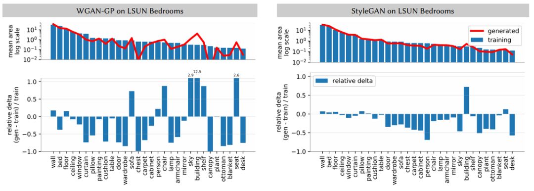
Because most categories do not appear in most images, the authors sorted the categories in descending order and then focused on the most common categories among them. This comparison can reveal many specific differences between many current best models. The two models analyzed were both trained on the same image distribution (LSUN bedroom set), but WGAN-GP had a much larger gap from the true distribution than StyleGAN.
It is also possible to summarize the statistical differences of the segmentation with a single numerical value. To do this, the authors defined the Frechet Segmentation Distance (FSD), which is similar to the commonly used Frechet Inception Distance (FID) metric, but FSD is interpretable:

Where, µ_t is the average pixel count for each object category on a training image sample, and Σ_t is the covariance of these pixel counts. Similarly, µ_g and Σ_g reflect the segmentation statistics of the generated model. In the experiments, the authors compared the statistics of 10,000 generated samples and 10,000 natural images.
Generated image segmentation statistics measure the entire distribution: for example, they can reveal cases where the generator ignores specific object categories. However, they do not individually exclude specific images that should have generated a certain object but did not. To gain further insights, a method to visualize the omissions of the generator on each image is needed.
Quantifying Mode Collapse at the Instance Level
To address the above issues, the authors compared image pairs (x, x’), where x is a real image (containing specific target categories missed by the GAN generator G), and x’ is a projection in the space of all images that can be generated by the GAN model layers.
-
Define a solvable inverse problem
Ideally, it should be possible to find an image perfectly synthesized by generator G, which is close to the real image x. Mathematically, the goal is to find  , where
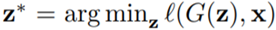 , l is the distance metric in image feature space. Unfortunately, due to the high number of layers in G, previous methods were unable to solve this complete inverse problem of the generator. Therefore, the authors turned to solving a solvable subproblem of this complete inverse problem. The authors decomposed the generator G into layers:
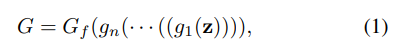
Where g_1, …, g_n are several early layers of the generator, and G_f is a combination of all later layers of G.
Any image that can be generated by G can also be generated by G_f. That is, if we denote the set of all images that can be output by G as range(G), then range(G) ⊂ range(G_f). In other words, G cannot generate any image that G_f cannot generate. Therefore, any omissions that can be determined in range(G_f) are also places omitted by range(G).
Thus, for layer-wise inverse propagation, the authors achieved visualization of omissions by more easily inversing the later layers of G_f:
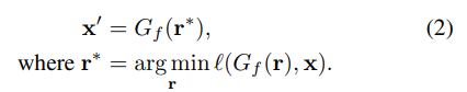
The authors stated that although the final goal is to find the intermediate representation r, starting from an estimated z can be very helpful: an initial estimate of z can assist in searching for better r values that are more likely to be generated by z. Therefore, the process of solving this inverse problem is divided into two steps: first, construct a neural network E to approximate the inverse of G, and compute an estimated result z_0 = E(x). Then, solve an optimization problem to determine an intermediate representation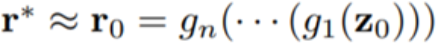 , which can generate a reconstructed image
  , to closely restore x. Figure 3 illustrates this layer-wise inverse propagation method.
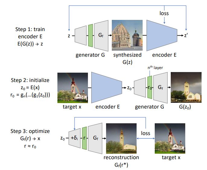
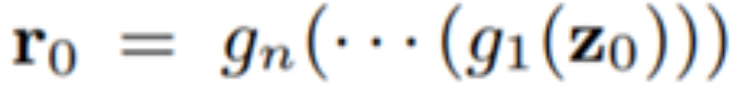 . Then use r_0 to initialize the search for r* to obtain a reconstruction x’ close to the target x.
-
Layer-wise Network Inversion
By pre-training individual layers on smaller problems, training deep networks becomes easier. Therefore, to learn the inverse neural network E, the authors chose a layer-wise execution method. For each layer g_i ∈ {g_1, …, g_n, G_f}, train a small network e_i to approximate the inverse of g_i. That is, define r_i = g_i(r_i−1), the goal is to learn a network e_i that can approximately compute r_{i−1} ≈ e_i(r_i). The authors also hope that the predictions of network e_i can well preserve the outputs of layer g_i, so it is required that r_i ≈ g_i(e_i(r_i)). The authors trained e_i by minimizing the left and right inverse propagation losses:
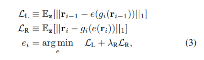
To focus the training on the manifold of representations obtained by the generator, the authors sampled z and calculated samples of r_{i−1} and r_i using layer g_i, thus r_{i−1} = g_{i−1}(· ·· g_1(z)· ··). Here ||·||_1 denotes L1 loss, and the authors set λ_R to 0.01 to emphasize the reconstruction of r_{i−1}.
Once all layers have completed their inversions, a network can be built for the entire G:

By jointly fine-tuning this network E* built for the overall inversion of G, further optimization can also be achieved. The authors denote the fine-tuned results as E.
Results
Figures 2 and 4 show the generated image segmentation statistics of WGAN-GP, StyleGAN, and Progressive GAN trained on the LSUN bedroom set.
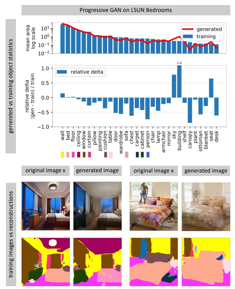
The histograms indicate that for various segmentation target categories, StyleGAN can better match the true distribution of these targets than Progressive GAN, while WGAN-GP matches the worst.
Table 1 summarizes these differences using the Frechet Segmentation Distance, confirming that better models overall match the segmentation statistics more closely with the true distribution.
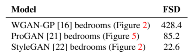
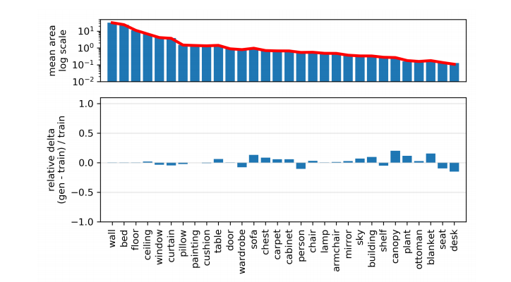
Figure 5 measured the sensitivity of the generated image segmentation statistics on a limited sample set of 10,000 images.
Figures 1 and 4 provide results of the analysis of generated segmentation statistics using the newly proposed method on the church and bedroom datasets. These histograms indicate that the generator partially skips difficult sub-tasks.
Figure 6 compares the new inverse method with previous inverse methods in the first three columns. The last three columns of Figure 6 compare the complete new method (f) with two versions of ablation experiments.
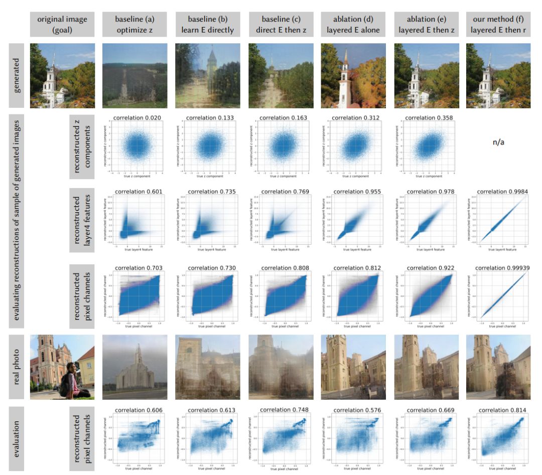
Figure 6: Comparing several methods of inverting the Progressive GAN generator on LSUN church images
The authors applied the above inverse tools to test the ability of various generators to synthesize images outside the training set. Figure 7 shows qualitative results of applying method (f) to invert and reconstruct natural photos of different scenes using the Progressive GAN trained on the LSUN bedroom set.
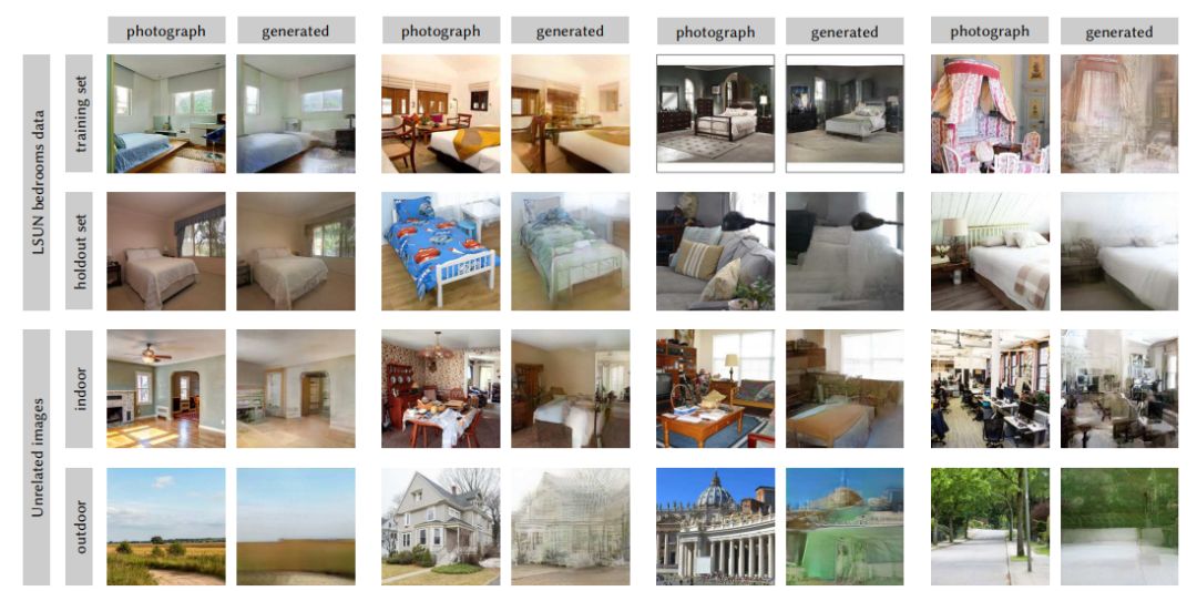
Figure 7: Inversion layer of the Progressive GAN bedroom image generator.
Figure 8 shows similar qualitative results obtained by the Progressive GAN trained on the LSUN church outdoor dataset.
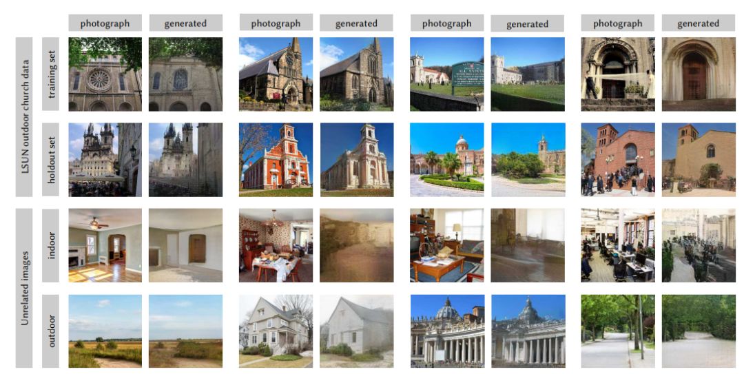
Figure 8: Inversion layer of the Progressive GAN outdoor generator.
——END——