Overview of Neural Network Activation Functions: From ReLU to GELU

Selected from | mlfromscratch

Author | Casper Hansen

Source | 机器之心

Contributors | 熊猫、杜伟

The importance of activation functions in neural networks is self-evident. Casper Hansen from the Technical University of Denmark introduces the sigmoid, ReLU, ELU, and the newer Leaky ReLU, SELU, and GELU activation functions through formulas, charts, and code experiments, comparing their advantages and disadvantages.

When calculating the activation values for each layer, we need to use the activation function to determine what these activation values actually are. Based on the activations, weights, and biases from the previous layer, we need to compute a value for each activation in the next layer. However, before sending that value to the next layer, we need to scale this output using an activation function. This article will introduce different activation functions. Before reading this article, you may want to check out my previous article on forward and backward propagation in neural networks, which briefly mentioned activation functions but did not explain what they actually do. The content of this article will build upon the knowledge you gained from the previous article.Previous article link: https://mlfromscratch.com/neural-networks-explained/Casper HansenTable of Contents

• Overview

• What is the sigmoid function?

• Gradient Issues: Backpropagation

• Gradient Vanishing Problem

• Gradient Explosion Problem

• Extreme Cases of Gradient Explosion

• Avoiding Gradient Explosion: Gradient Clipping/Norm

• Rectified Linear Unit (ReLU)

• Dead ReLU: Advantages and Disadvantages

• Exponential Linear Unit (ELU)

• Leaky Rectified Linear Unit (Leaky ReLU)

• Scaled Exponential Linear Unit (SELU)

• SELU: A Special Case of Normalization

• Weight Initialization + Dropout

• Gaussian Error Linear Unit (GELU)

• Code: Hyperparameter Search for Deep Neural Networks

• Further Reading: Books and Papers

OverviewActivation functions are a crucial part of neural networks. In this lengthy article, I will comprehensively cover six different activation functions and explain their respective advantages and disadvantages. I will provide the equations and differential equations for these activation functions, along with their illustrations. The goal of this article is to explain these equations and graphs in simple terms. I will introduce the gradient vanishing and explosion problems; for the latter, I will explain the causes of gradient explosion using the excellent example proposed by Nielsen. Finally, I will provide some code so you can run experiments in Jupyter Notebook.

I will perform some small code experiments on the MNIST dataset to obtain loss and accuracy graphs for each activation function.

What is the sigmoid function?The sigmoid function is a logistic function, meaning that regardless of the input, the output will always be between 0 and 1. In other words, every neuron, node, or activation you input will be scaled to a value between 0 and 1.

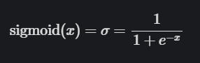
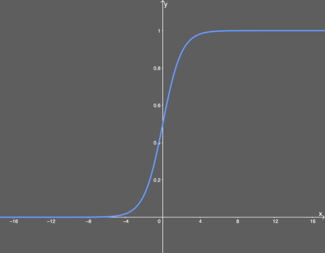
Illustration of the sigmoid function.Functions like the sigmoid are often referred to as nonlinear functions because we cannot describe them using linear terms. Many activation functions are nonlinear or a combination of linear and nonlinear (though cases where part of the function is linear are rare). This is generally not a problem, except when the value is exactly 0 or 1 (which can sometimes happen). Why is this a problem? This issue is related to backpropagation (for an introduction to backpropagation, see my previous article). In backpropagation, we need to calculate the gradient for each weight, which means small updates for each weight. The purpose of this is to optimize the output of activation values across the network so that better results can be achieved at the output layer, thereby optimizing the cost function. During backpropagation, we have to calculate how each weight affects the cost function, specifically by calculating the partial derivative of the cost function with respect to each weight. Suppose we do not define a single weight but define all weights w in the last layer L as w^L, their derivatives would be: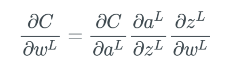Note that when calculating the partial derivative, we need to find the equation for ∂a^L and then only differentiate ∂z^L while keeping the rest unchanged. We use the prime symbol “‘” to denote the derivative of any function. When calculating the partial derivative of the intermediate term ∂a^L/∂z^L, we have:The derivative of the sigmoid function is: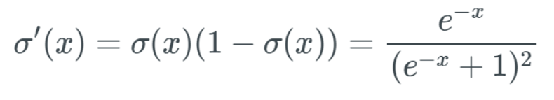When we input a very large x value (positive or negative) into this sigmoid function, we get a y value that is almost 0—meaning that when we input w×a+b, we might get a value close to 0.

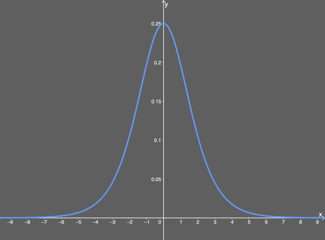
Illustration of the derivative of the sigmoid function. When x is a very large value (positive or negative), we are essentially multiplying this almost 0 value by the rest of the partial derivative.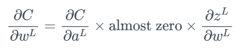If too many weights have such large values, we simply cannot get a network that can adjust the weights, which is a big problem. If we do not adjust these weights, then the network will only have minor updates, and the algorithm cannot bring about much improvement to the network over time. For each computation of the partial derivative for a specific weight, we put it into a gradient vector, and we will use this gradient vector to update the neural network. You can imagine that if all values in the gradient vector are close to 0, we cannot really update anything at all.This describes the gradient vanishing problem. This problem makes the sigmoid function impractical in neural networks, and we should use other activation functions introduced later.Gradient IssuesGradient Vanishing ProblemAs mentioned in my previous article, if we want to update a specific weight, the update rule is: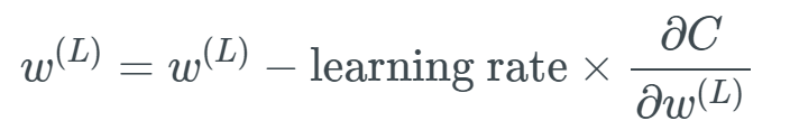But what if the partial derivative ∂C/∂w^(L) is very small, as if it has vanished? This is when we encounter the gradient vanishing problem, where many weights and biases can only receive very small updates.

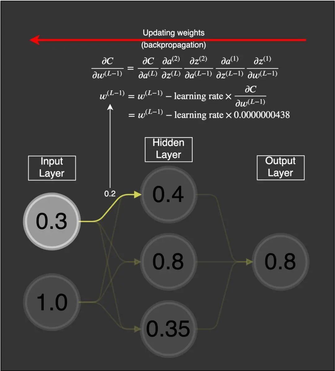
As you can see, if the value of the weight is 0.2, when the gradient vanishing problem occurs, this value will hardly change. Since this weight connects the first neuron of the first layer to the first neuron of the second layer, we can represent it as

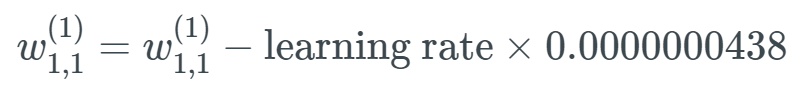
Assuming this weight’s value is 0.2, given a learning rate (the exact value does not matter, I used 0.5 here), the new weight will be:

This weight was originally 0.2, and now it has been updated to 0.199999978. Clearly, this is a problem: the gradient is very small, as if it has vanished, causing the weights in the neural network to hardly update. This can lead to the nodes in the network being far from their optimal values. This problem severely hinders the learning of neural networks. It has been observed that if different layers learn at different speeds, this problem can become even more severe. Layers learn at different speeds, and the earlier layers always become worse based on the learning rate.

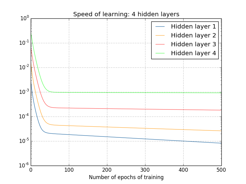
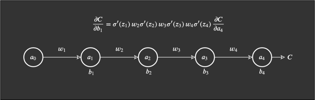
From Nielsen’s book “Neural Networks and Deep Learning”. In this example, the learning speed of hidden layer 4 is the fastest, as its cost function only depends on the weight changes connected to hidden layer 4. Let’s look at hidden layer 1; here the cost function depends on the weight changes connecting hidden layer 1 with hidden layers 2, 3, and 4. If you’ve read the content about backpropagation in my previous article, you may know that earlier layers in the network reuse calculations from later layers.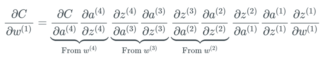At the same time, as previously mentioned, the last layer only depends on a set of changes that occur when calculating the partial derivative: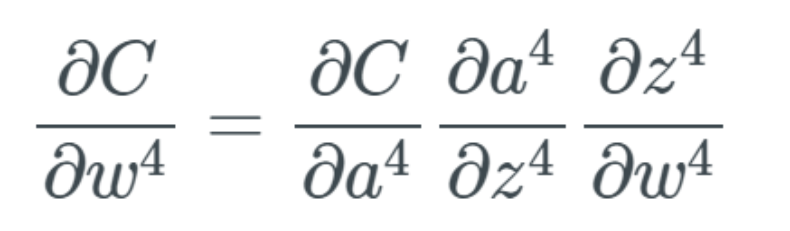Ultimately, this becomes a big problem because now the learning speeds of the weight layers differ. This means that the layers further back in the network will almost certainly be optimized more by the layers closer to the front of the network. Moreover, the problem is that the backpropagation algorithm does not know in which direction to pass the weights to optimize the cost function.Gradient Explosion ProblemThe gradient explosion problem is essentially the opposite of the gradient vanishing problem. Research has shown that such issues can occur, where the weights are in a “blown up” state, meaning their values rapidly increase.

We will illustrate this with the following example:

• http://neuralnetworksanddeeplearning.com/chap5.html#what’s_causing_the_vanishing_gradient_problem_unstable_gradients_in_deep_neural_nets

Note that this example can also be used to demonstrate the gradient vanishing problem, and I chose it from a more conceptual perspective for easier explanation. Essentially, when 0<w<1, we may encounter the gradient vanishing problem; when w>1, we may encounter the gradient explosion problem. However, when a layer encounters this problem, there are likely to be more weights that meet the conditions for gradient vanishing or explosion. We start with a simple network. This network has a small number of weights, biases, and activations, and each layer only has one node.This network is simple. Weights are represented as w_j, biases as b_j, and the cost function as C. Nodes, neurons, or activations are represented as circles. Nielsen used the common physical representation Δ to describe changes in a value (this is different from the gradient symbol ∇). For example, Δb_j describes the change in the value of the j-th bias.The core of my previous article was that we need to measure the rate of change of weights and biases related to the cost function. Ignoring layers for now, let’s look at a specific bias, which is the first bias b_1. We then measure the rate of change using the following formula: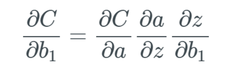The arguments of the formula below are the same as the partial derivatives above. How do we measure the rate of change of the cost function based on the rate of change of the bias? As introduced just now, Nielsen used Δ to describe changes, so we can say that this partial derivative can roughly be replaced by Δ: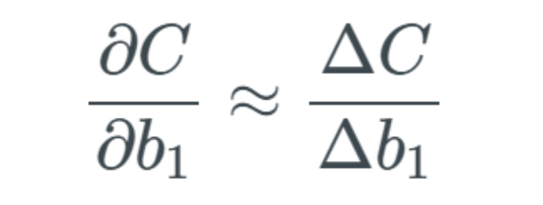The changes in weights and biases can be visualized as follows:

The animation is from 3blue1brown, video link:https://www.youtube.com/watch?v=tIeHLnjs5U8.We start from the starting point of the network and calculate how changes in the first bias b_1 will affect the network. Since we know from the previous article that the first bias b_1 feeds into the first activation a_1, we start from here. Let’s review this equation: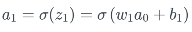If b_1 changes, we represent this change as Δb_1. Therefore, we note that when b_1 changes, the activation a_1 also changes—we usually represent this as ∂a_1/∂b_1. Thus, we have the expression for the partial derivative on the left, which is the change in a_1 related to b_1. But we start replacing the left-hand terms, first replacing a_1 with the sigmoid of z_1: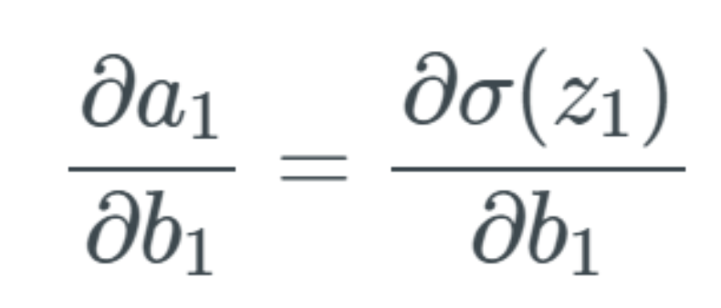The above equation indicates that when b_1 changes, there is a change in the activation value a_1. We describe this change as Δa_1. We consider the change Δa_1 to be approximately equal to the change in the activation value a_1 plus the change Δb_1.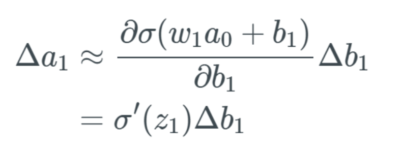Here we skipped a step, but essentially we just computed the partial derivative and replaced the fraction part with the result of the partial derivative.The change in a_1 leads to a change in z_2The change described by Δa_1 will now lead to a change in the input z_2 of the next layer. If this seems strange or you are not convinced, I suggest you read my previous article.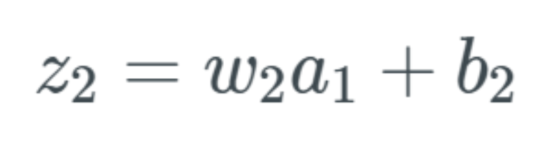Using the same notation, we denote the next change as Δz_2. We will have to go through the previous process again, but this time we need to obtain the change in z_2: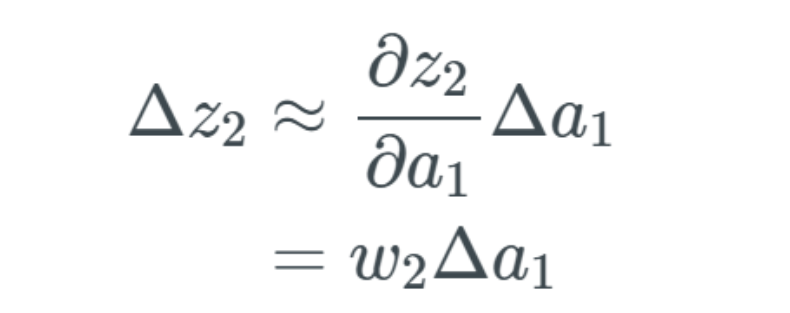We can use the following to replace Δa_1:We only compute this expression. I hope you clearly understand the process up to this point—this is similar to the process of calculating Δa_1. This process will repeat until we compute the entire network. By replacing Δa_j values, we obtain a final function that calculates the changes related to the cost function across the entire network (i.e., all weights, biases, and activations).

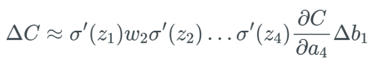
Based on this, we then calculate ∂C/∂b_1 to obtain the final expression we need: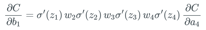Extreme Cases of Gradient ExplosionAccordingly, if all weights w_j are very large, meaning that many weights have values greater than 1, we will begin to multiply by larger values. For example, if all weights have some very high values like 100, and we get some random output from the sigmoid function’s derivative between 0 and 0.25: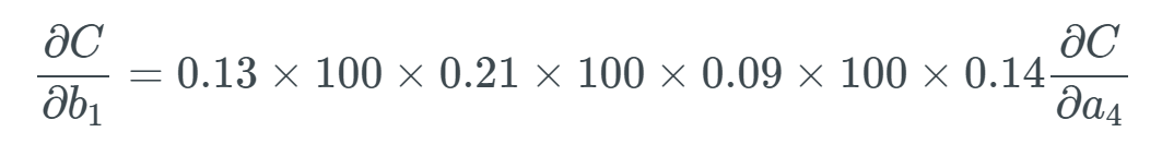The last partial derivative is 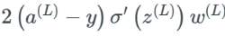, and it is reasonable to believe this will be far greater than 1, but for the sake of example, we will set it to 1.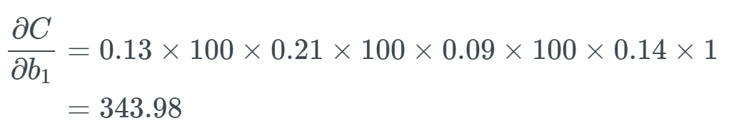Using this update rule, if we assume b_1 was previously equal to 1.56 and the learning rate is 0.5.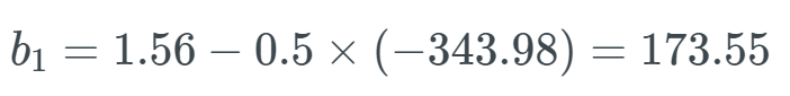Even though this is an extreme case, you get my point. The values of weights and biases can explode, leading to an explosion across the entire network.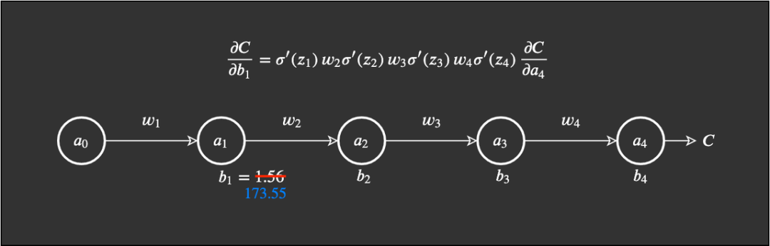Now take a moment to think about the weights and biases of the network and other parts of the activation, exploding their values. This is what we refer to as the gradient explosion problem. Clearly, such a network learns nothing, so this will completely ruin the task you are trying to solve.Avoiding Gradient Explosion: Gradient Clipping/NormThe basic idea for solving the gradient explosion problem is to set a rule for it. I won’t delve into the mathematical explanation here, but I will give the steps for this process:

• Select a threshold—if the gradient exceeds this value, use gradient clipping or gradient norm;

• Define whether to use gradient clipping or norm. If using gradient clipping, you specify a threshold, such as 0.5. If this gradient value exceeds 0.5 or -0.5, then either scale it to the threshold range through gradient normalization or clip it to the threshold range.

However, note that these gradient methods cannot avoid the gradient vanishing problem. Therefore, we will further explore more methods to solve this problem. Generally speaking, if you are using recurrent neural network architectures (like LSTM or GRU), then you will need these methods because this architecture often encounters gradient explosion situations.Rectified Linear Unit (ReLU)The Rectified Linear Unit is our method for solving the gradient vanishing problem, but does this lead to other issues? Please read on. The formula for ReLU is as follows:

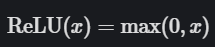
The ReLU formula states:

• If the input x is less than 0, the output equals 0;

• If the input x is greater than 0, the output equals the input.

This is good, but how does it relate to the gradient vanishing problem? First, we need to get its differential equation: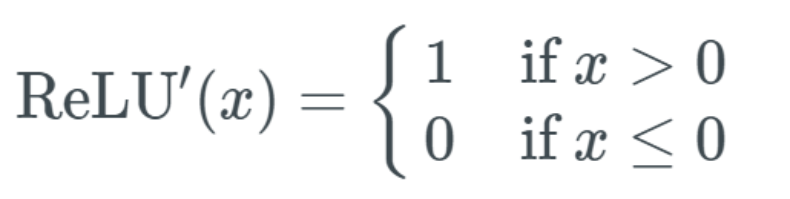This means:

• If the input x is greater than 0, the output equals 1;

• If the input is less than or equal to 0, the output becomes 0.

Using the following graph:

Differentiated ReLU.Now we have the answer: when using the ReLU activation function, we do not get very small values (like the 0.0000000438 from the sigmoid function earlier). Instead, it is either 0 (leading to some gradients not returning anything) or 1. But this gives rise to another problem: the dead ReLU problem. What happens if there are too many values below 0 when calculating the gradient? We will get quite a few weights and biases that will not update because their update amount is 0. To understand how this process performs in practice, let’s look back at the earlier example of gradient explosion. In this equation, we denote ReLU as R, and we only need to replace each sigmoid σ with R: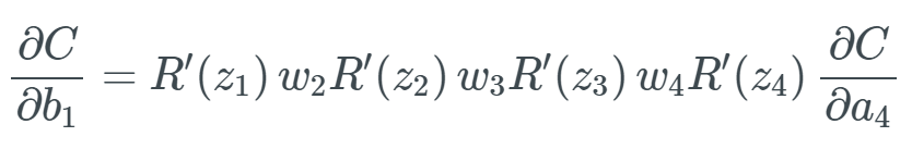Now, suppose that a random input z of the differentiated ReLU is less than 0—this function will cause the bias to “die”. Assume it is R'(z_3)=0: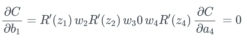Conversely, when we get R'(z_3)=0, multiplying by other values naturally yields 0, which will lead to this bias dying. We know that the new value of a bias is that bias minus the learning rate times the gradient, which means we get an update of 0.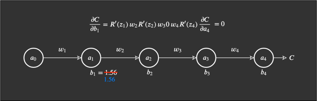Dead ReLU: Advantages and DisadvantagesWhen we introduce the ReLU function into neural networks, we also introduce a lot of sparsity. So what does the term sparsity mean? Sparsity: a small number, usually dispersed over a large area. In neural networks, this means that the activation matrix contains many 0s. What does this sparsity allow us to achieve? When a certain proportion (say 50%) of activations saturate, we call this neural network sparse. This can enhance efficiency in terms of time and space complexity—constant values (typically) require less space and lower computational costs. Yoshua Bengio and others found that this component of ReLU can actually improve the performance of neural networks, along with the previously mentioned efficiency in time and space.Paper link: https://www.utc.fr/~bordesan/dokuwiki/_media/en/glorot10nipsworkshop.pdf Advantages:

• Compared to sigmoid, due to sparsity, lower time and space complexity; no costlier exponential calculations;

• Avoids gradient vanishing problem.

Disadvantages:

• Introduces the dead ReLU problem, meaning that most components of the network will never update. However, this can sometimes also be an advantage;

• ReLU cannot avoid the gradient explosion problem.

Exponential Linear Unit (ELU)The Exponential Linear Unit activation function solves some of the problems of ReLU while retaining some of its good aspects. This activation function requires selecting an α value; common values range from 0.1 to 0.3. If you’re not good at math, the formula for ELU may seem a bit difficult to understand: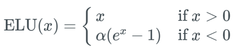Let me explain. If your input x value is greater than 0, the result is the same as ReLU—i.e., the y value equals the x value; but if the input x value is less than 0, we will get a value slightly less than 0. The y value obtained depends on the input x value but must also consider the parameter α—you can adjust this parameter as needed. Furthermore, we introduce the exponential operation e^x, so the computational cost of ELU is higher than that of ReLU. Below is a graph of the ELU function with an α value of 0.2:

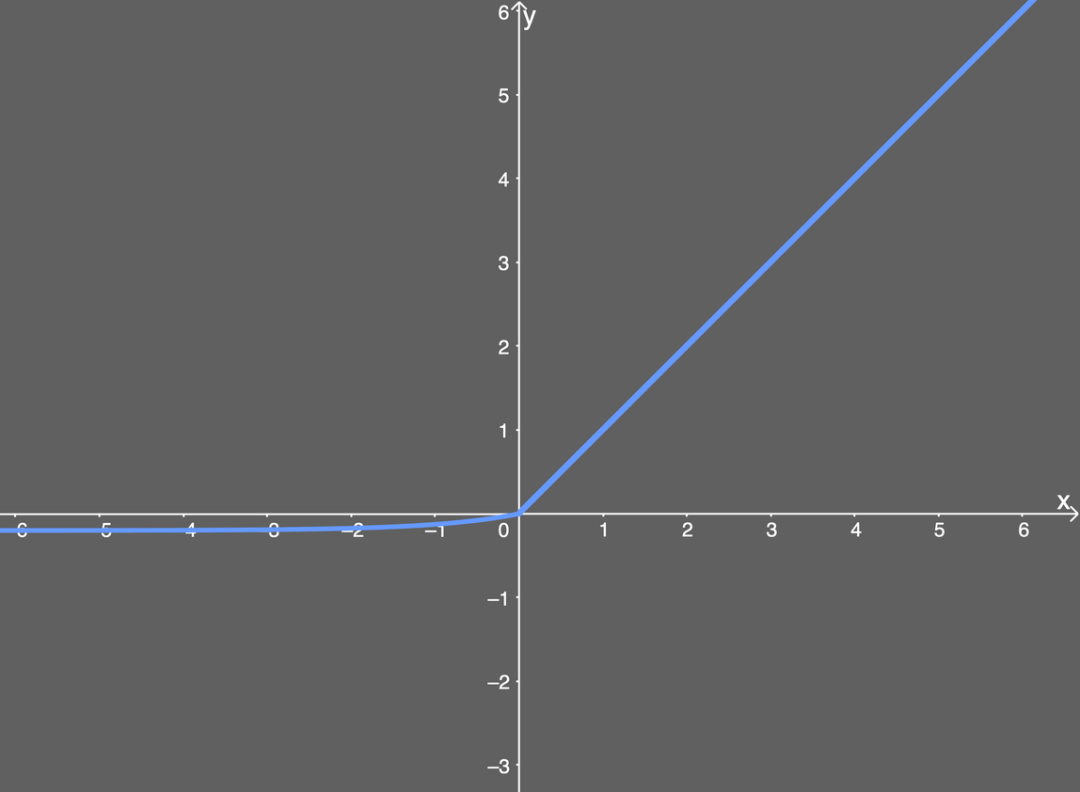
Illustration of the ELU activation function.The above graph is intuitive, and we should still be able to handle the gradient vanishing problem well, as the input values are not mapped to very small output values. But what about the derivative of ELU? That is also very important.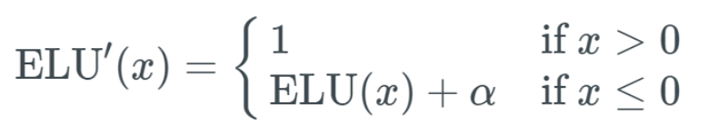It looks quite simple. If the input x is greater than 0, the output is 1; if the input x is less than or equal to 0, the output is the ELU function (not differentiated) plus the α value. The graph can be drawn as:

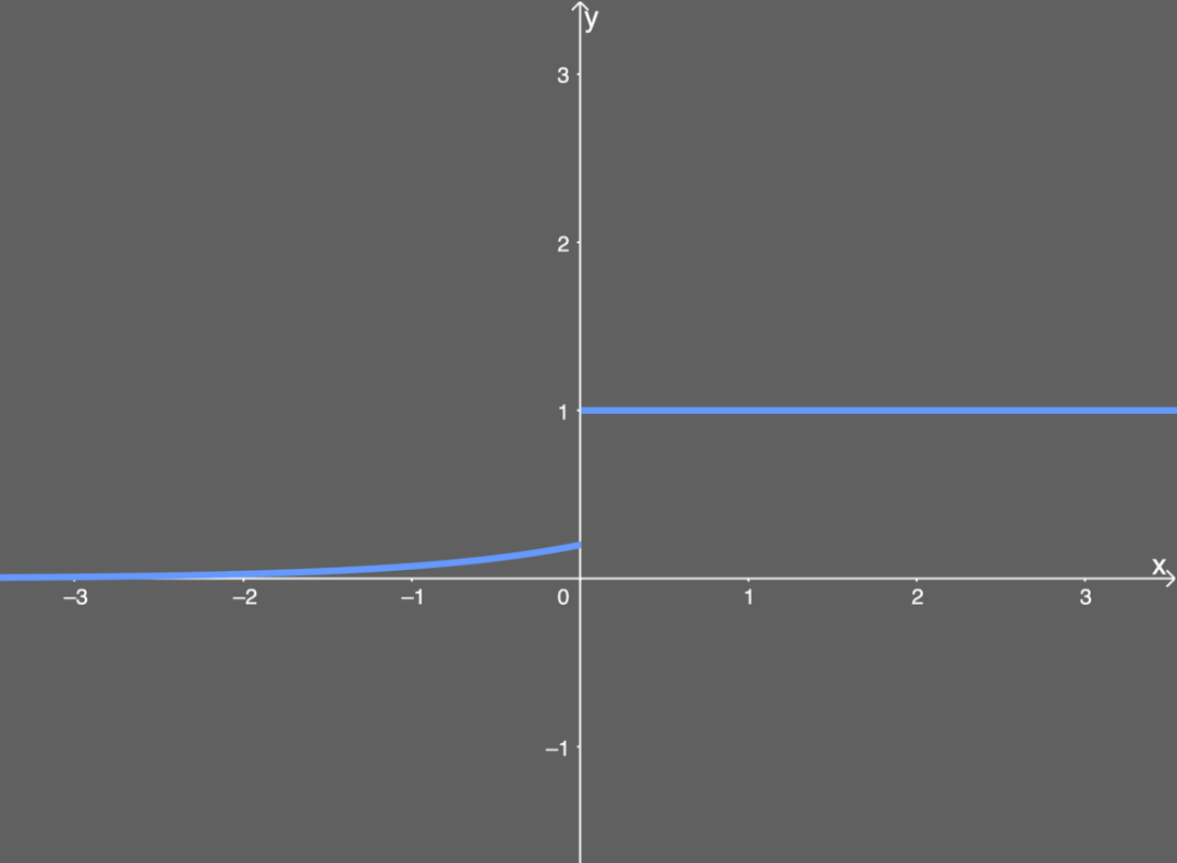
Differentiated ELU activation function.You may have noticed that this successfully avoids the dead ReLU problem while still retaining some of the computational speed advantages of the ReLU activation function—meaning that there are still some dead components in the network. Advantages:

• Avoids the dead ReLU problem;

• Can produce negative outputs, which can help push weights and biases in the right direction;

• Can obtain activations during gradient computation instead of letting them equal 0.

Disadvantages:

• Due to the inclusion of exponential operations, the computation time is longer;

• Cannot avoid the gradient explosion problem;

• The neural network does not learn the α value.

Leaky Rectified Linear Unit Activation Function (Leaky ReLU)

The Leaky Rectified Linear Unit activation function also has an α value, typically ranging from 0.1 to 0.3. Leaky ReLU is commonly used but has some disadvantages compared to ELU while also having some advantages over ReLU. The mathematical form of Leaky ReLU is as follows: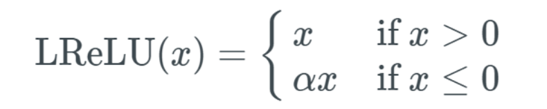Therefore, if the input x is greater than 0, the output is x; if the input x is less than or equal to 0, the output is α multiplied by the input. This means it can solve the dead ReLU problem because the gradient value is no longer limited to 0—additionally, this function can avoid the gradient vanishing problem. Although the gradient explosion problem still exists, the code section later will show how to address this. Below is an illustration of Leaky ReLU, assuming an α value of 0.2:

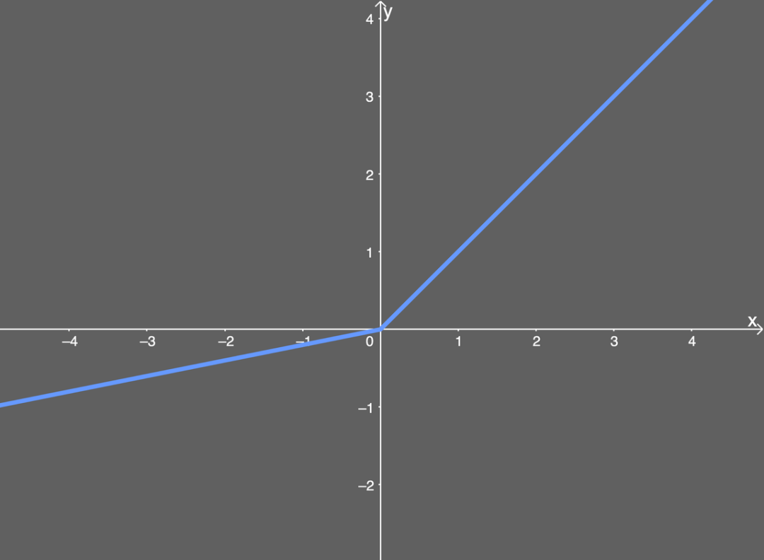
Illustration of Leaky ReLU.As seen in the formula, if the x value is greater than 0, any x value maps to the same y value; but if the x value is less than 0, there will be an additional coefficient of 0.2. In other words, if the input value x is -5, the mapped output value will be -1. Because the Leaky ReLU function is a combination of two linear parts, its derivative is quite simple: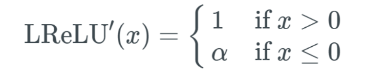The first linear part is when x is greater than 0, the output is 1; while when the input is less than 0, the output is the α value, which we choose to be 0.2.

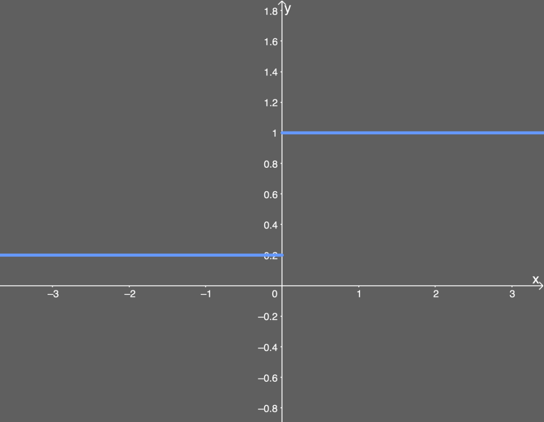
Illustration of differentiated Leaky ReLU.It is also clear from the above graph that for inputs x greater than or less than 0, the differentiated Leaky ReLU is a constant. Advantages:

• Similar to ELU, Leaky ReLU can also avoid the dead ReLU problem because it allows smaller gradients during derivative calculations;

• Since it does not include exponential operations, the computation speed is faster than ELU.

Disadvantages:

• Cannot avoid the gradient explosion problem;

• The neural network does not learn the α value;

• In differentiation, both parts are linear; while ELU has one part linear and one part nonlinear.

Scaled Exponential Linear Unit Activation Function (SELU)The Scaled Exponential Linear Unit activation function is relatively new, and the paper introducing it contains a 90-page appendix (including theorems and proofs). When applying this activation function in practice, it is essential to use lecun_normal for weight initialization. If dropout is to be applied, a special version called AlphaDropout should be used. The code section later will describe this in more detail. The authors of the paper have calculated two values for the formula: α and λ, as follows: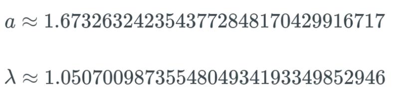As you can see, they have many decimal places for absolute precision. Moreover, they are predetermined, meaning we do not have to worry about how to choose a suitable α value for this activation function. To be honest, this formula looks somewhat similar to other formulas. All new activation functions seem like combinations of existing activation functions. The formula for SELU is as follows: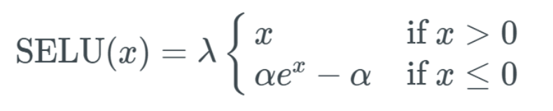That is to say, if the input value x is greater than 0, the output value is x multiplied by λ; if the input value x is less than 0, it will get a singular function that increases as x increases and approaches the value 0.0848 when x is 0. Essentially, when x is less than 0, we first use α multiplied by the exponential of x, then subtract α and multiply by λ.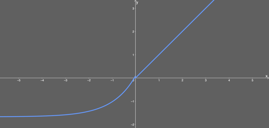Illustration of the SELU function.Special Case of SELUSELU activation can perform self-normalization in neural networks. What does this mean? First, let’s look at what normalization is. Simply put, normalization first subtracts the mean and then divides by the standard deviation. Therefore, after normalization, the components of the network (weights, biases, and activations) have a mean of 0 and a standard deviation of 1. This is exactly the output value of the SELU activation function. What does it mean for the mean to be 0 and the standard deviation to be 1? Under the assumption that the initialization function is lecun_normal, the network parameters will be initialized to a normal distribution (or Gaussian distribution), and under SELU, the network will be completely normalized within the range described in the paper. Essentially, when multiplying or adding such network components, the network is still considered to conform to a Gaussian distribution. We call this normalization. Conversely, this also means that the entire network and its final output layer are also normalized. What does a normal distribution with mean μ of 0 and variance ν of 1 look like?The output of SELU is normalized, which can be referred to as internal normalization; therefore, in fact, all outputs are mean 0 and standard deviation 1. This is different from external normalization, which would use batch normalization or other methods. Great, this means all components will be normalized. But how is this achieved? To briefly explain, when the input is less than 0, the variance decreases; when the input is greater than 0, the variance increases—and the standard deviation is the square root of the variance, so we make the standard deviation equal to 1. We obtain zero mean through gradients. We need some positive and negative values to make the mean 0. My previous article mentioned that gradients can adjust the weights and biases of the neural network, so we need these gradients to output some negative and positive values to control the mean. The main function of the mean μ and variance ν is to provide us with a domain Ω, allowing us to always map the mean and variance to predefined intervals. These intervals are defined as follows: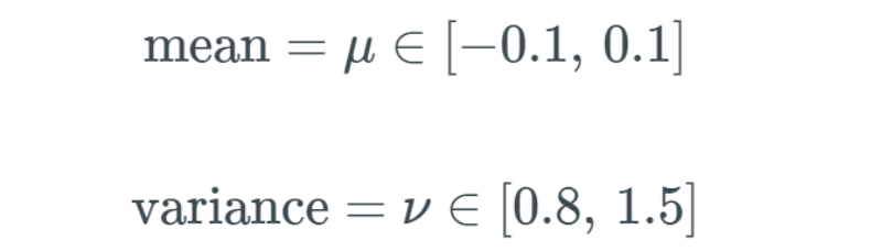∈ symbol indicates that the mean and variance are within these predefined intervals. Conversely, this can prevent the network from experiencing gradient vanishing and explosion problems. Below, I quote a passage from the paper explaining how they derived this activation function, which I think is important:

SELU allows the construction of a mapping g whose properties can achieve SNN (self-normalizing neural networks). SNN cannot be achieved through (scaled) rectified linear units (ReLU), sigmoid units, tanh units, or Leaky ReLU. This activation function needs: (1) negative and positive values to control the mean; (2) saturation regions (where the derivative approaches zero) to suppress larger variances in lower layers; (3) slopes greater than 1 to increase variance when the variance is too small in lower layers; (4) a continuous curve. The latter ensures a fixed point where variance suppression can be balanced by variance increase. We can satisfy these properties of the activation function by multiplying by the exponential linear unit (ELU), and λ>1 ensures that the slope of the net input of positive values is greater than 1.

Now let’s look at the differential function of SELU: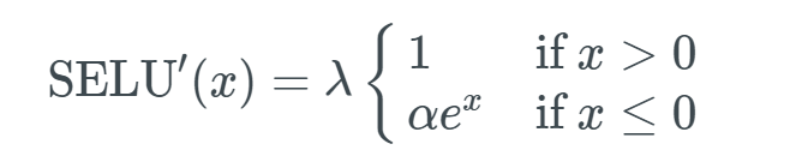Great, not too complicated; we can simply explain. If x is greater than 0, the output value is λ; if x is less than 0, the output is α multiplied by the exponential of x, then multiplied by λ. Its graph looks special:

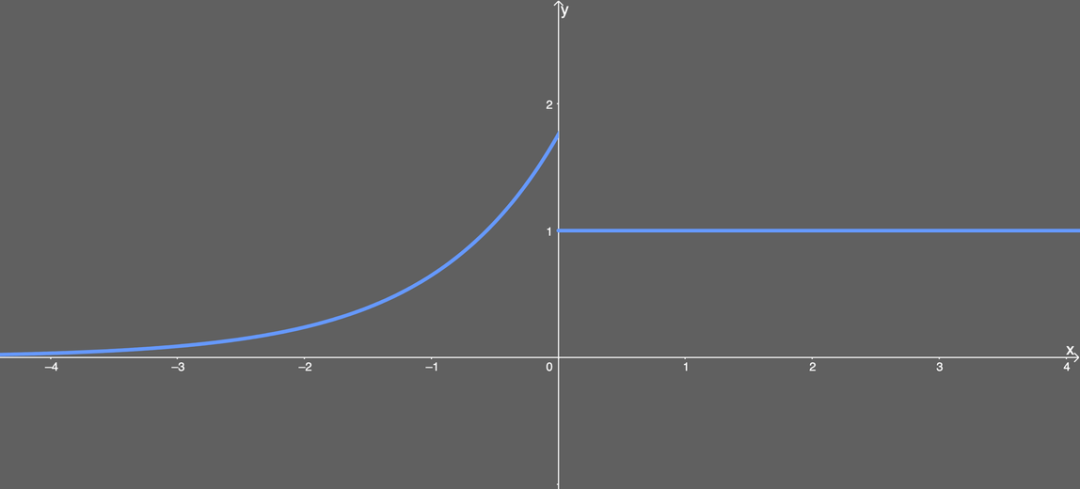
Illustration of differentiated SELU function.Note that the SELU function also requires lecun_normal for weight initialization; and if you wish to use dropout, you must also use a special version called Alpha Dropout. Advantages:

• Internal normalization is faster than external normalization, meaning the network can converge faster;

• Gradient vanishing or explosion problems cannot occur, see theorems 2 and 3 in the appendix of the SELU paper.

Disadvantages:

• This activation function is relatively new—more comparative exploration of its application in architectures like CNN and RNN is needed.

• Here is a paper using SELU in CNN: https://arxiv.org/pdf/1905.01338.pdf

GELUThe Gaussian Error Linear Unit activation function has been applied in recent transformer models (Google’s BERT and OpenAI’s GPT-2). The GELU paper dates back to 2016, but it has only recently gained attention. The form of this activation function is: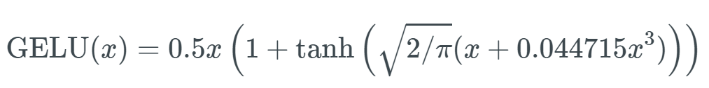It can be seen that this is a combination of some functions (like the hyperbolic tangent function tanh) with approximate values. There is not much more to say. Interestingly, the graph of this function:

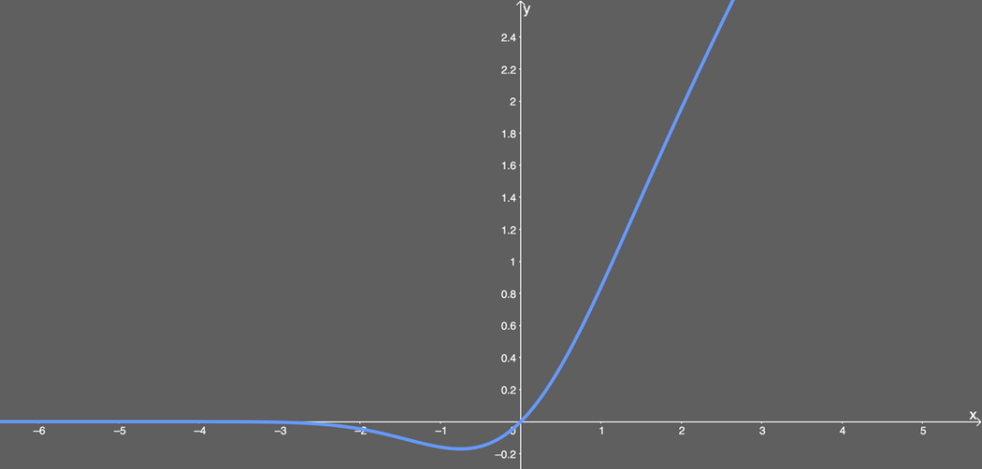
Illustration of GELU activation function.It can be seen that when x is greater than 0, the output is x; but in the interval from x=0 to x=1, the curve is more biased towards the y-axis. I could not find the derivative of this function, so I used WolframAlpha to differentiate this function. The result is as follows: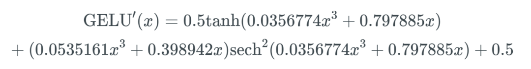As before, this is another form of hyperbolic function combination. But its graph looks interesting:

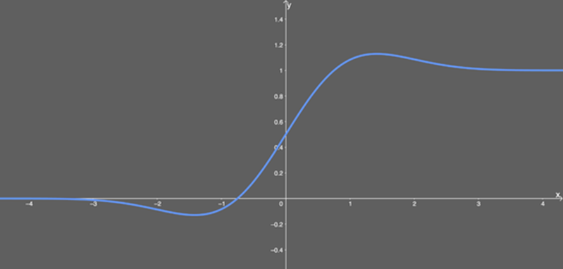
Illustration of differentiated GELU activation function.Advantages:

• Seems to be the current best in the field of NLP; especially performs best in transformer models;

• Avoids the gradient vanishing problem.

Disadvantages:

• Although proposed in 2016, it is still a relatively novel activation function in practical applications.

Code for Deep Neural NetworksSuppose you want to try all these activation functions to see which one is the best for you; how would you do that? Usually, we perform hyperparameter optimization—which can be achieved using the GridSearchCV function from scikit-learn. However, we want to make comparisons, so our idea is to select some hyperparameters and keep them constant while modifying the activation function. Let me explain what I am going to do:

• Train the same neural network model using the activation functions mentioned in this article;

• Using the history of each activation function, plot the graphs of loss and accuracy over epochs.

This code is also published on GitHub and supports Colab so that you can run it quickly. The link is: https://github.com/casperbh96/Activation-Functions-Search I prefer using Keras’s high-level API, so this will be done using Keras. First, import everything we need. Note that here we use 4 libraries: tensorflow, numpy, matplotlib, keras.

import tensorflow as tf
import numpy as np
import matplotlib.pyplot as plt
from keras.datasets import mnist
from keras.utils.np_utils import to_categorical
from keras.models import Sequential
from keras.layers import Dense, Dropout, Flatten, Conv2D, MaxPooling2D, Activation, LeakyReLU
from keras.layers.noise import AlphaDropout
from keras.utils.generic_utils import get_custom_objects
from keras import backend as K
from keras.optimizers import Adam

Now load the dataset we need for our experiments; here we choose the MNIST dataset. We can import it directly from Keras.

(x_train, y_train), (x_test, y_test) = mnist.load_data()

Great, but we want to preprocess the data a bit, like normalizing it. We need to go through many functions to do this, mainly adjusting the image size (.reshape) and dividing by the maximum RGB value of 255 ( /= 255). Finally, we perform one-hot encoding on the data using to_categorical().

def preprocess_mnist(x_train, y_train, x_test, y_test):
    # Normalizing all images of 28x28 pixels
    x_train = x_train.reshape(x_train.shape[0], 28, 28, 1)
    x_test = x_test.reshape(x_test.shape[0], 28, 28, 1)
    input_shape = (28, 28, 1)

    # Float values for division
    x_train = x_train.astype('float32')
    x_test = x_test.astype('float32')

    # Normalizing the RGB codes by dividing it to the max RGB value
    x_train /= 255
    x_test /= 255

    # Categorical y values
    y_train = to_categorical(y_train)
    y_test= to_categorical(y_test)

    return x_train, y_train, x_test, y_test, input_shape

x_train, y_train, x_test, y_test, input_shape = preprocess_mnist(x_train, y_train, x_test, y_test)

Now that we have completed the data preprocessing, we can build the model and define the parameters required for Keras to run. First, we start with the convolutional neural network model itself. The SELU activation function is a special case; we need to use the kernel initializer ‘lecun_normal’ and a special form of dropout AlphaDropout(), while everything else remains standard settings.

def build_cnn(activation,
              dropout_rate,
              optimizer):
    model = Sequential()if(activation == 'selu'):
        model.add(Conv2D(32, kernel_size=(3, 3),
                  activation=activation,
                  input_shape=input_shape,
                  kernel_initializer='lecun_normal'))
        model.add(Conv2D(64, (3, 3), activation=activation, 
                         kernel_initializer='lecun_normal'))
        model.add(MaxPooling2D(pool_size=(2, 2)))
        model.add(AlphaDropout(0.25))
        model.add(Flatten())
        model.add(Dense(128, activation=activation, 
                        kernel_initializer='lecun_normal'))
        model.add(AlphaDropout(0.5))
        model.add(Dense(10, activation='softmax'))else:
        model.add(Conv2D(32, kernel_size=(3, 3),
                  activation=activation,
                  input_shape=input_shape))
        model.add(Conv2D(64, (3, 3), activation=activation))
        model.add(MaxPooling2D(pool_size=(2, 2)))
        model.add(Dropout(0.25))
        model.add(Flatten())
        model.add(Dense(128, activation=activation))
        model.add(Dropout(0.5))
        model.add(Dense(10, activation='softmax'))

    model.compile(
        loss='binary_crossentropy', 
        optimizer=optimizer, 
        metrics=['accuracy'])return model

Using the GELU function has a small problem; currently, Keras does not have this function. Fortunately, we can easily add new activation functions to Keras.

# Add the GELU function to Keras
def gelu(x):
    return 0.5 * x * (1 + tf.tanh(tf.sqrt(2 / np.pi) * (x + 0.044715 * tf.pow(x, 3))))
get_custom_objects().update({'gelu': Activation(gelu)})

# Add leaky-relu so we can use it as a string
get_custom_objects().update({'leaky-relu': Activation(LeakyReLU(alpha=0.2))})

act_func = ['sigmoid', 'relu', 'elu', 'leaky-relu', 'selu', 'gelu']

Now we can train the model using the different activation functions defined in the act_func array. We will run a simple for loop on each activation function and append the results to an array:

result = []for activation in act_func:print('\nTraining with -->{0}<-- activation function\n'.format(activation))

    model = build_cnn(activation=activation,
                      dropout_rate=0.2,
                      optimizer=Adam(clipvalue=0.5))

    history = model.fit(x_train, y_train,
          validation_split=0.20,
          batch_size=128, # 128 is faster, but less accurate. 16/32 recommended
          epochs=100,
          verbose=1,
          validation_data=(x_test, y_test))

    result.append(history)

    K.clear_session()del model
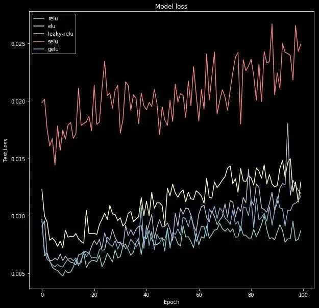
print(result)

Based on this, we can plot the graphs of loss and accuracy obtained from model.fit() for each activation function and see how the results change. Now we can plot the data; I wrote a small piece of code using matplotlib:

new_act_arr = act_func[1:]
ew_results = result[1:]def plot_act_func_results(results, activation_functions = []):
    plt.figure(figsize=(10,10))
    plt.style.use('dark_background')# Plot validation accuracy valuesfor act_func in results:
        plt.plot(act_func.history['val_acc'])

    plt.title('Model accuracy')
    plt.ylabel('Test Accuracy')
    plt.xlabel('Epoch')
    plt.legend(activation_functions)
    plt.show()# Plot validation loss values
    plt.figure(figsize=(10,10))for act_func in results:
        plt.plot(act_func.history['val_loss'])

    plt.title('Model loss')
    plt.ylabel('Test Loss')
    plt.xlabel('Epoch')
    plt.legend(activation_functions)
    plt.show()

plot_act_func_results(new_results, new_act_arr)

This will produce the following charts: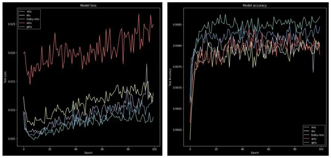Further ReadingBelow are four excellently written books:

• Deep Learning, Authors: Ian Goodfellow, Yoshua Bengio, Aaron Courville

• The Hundred-Page Machine Learning Book, Author: Andriy Burkov

• Hands-On Machine Learning with Scikit-Learn and TensorFlow, Author: Aurélien Géron

• Machine Learning: A Probabilistic Perspective, Author: Kevin P. Murphy

Below are the important papers discussed in this article:

• Leaky ReLU paper: https://ai.stanford.edu/~amaas/papers/relu_hybrid_icml2013_final.pdf

• ELU paper: https://arxiv.org/pdf/1511.07289.pdf

• SELU paper: https://arxiv.org/pdf/1706.02515.pdf

• GELU paper: https://arxiv.org/pdf/1606.08415.pdf