Neural Operators for Accelerating Scientific Simulations and Design

Introduction

In the unprecedented wave of artificial intelligence (AI) today, people cannot help but worry whether their jobs will gradually be replaced by AI, while exploratory scientists are trying to let AI replace themselves. Is it possible for AI to conduct scientific research? How can AI scientists help drive scientific exploration? The usual steps in scientific research include observation, hypothesis formulation, and experimental validation. In many fields, validation experiments are extremely tedious and slow, which greatly limits the productivity of modern scientific research and industry. If expensive experiments can be reliably replaced by computational simulations, it will lower the financial and resource thresholds, greatly expanding the hypothesis space that can be explored, making the 21st century a true historical moment of “technological explosion.” In the viewpoint article “Neural Operators for Accelerating Scientific Simulations and Design” published in 2024 in Nature Reviews Physics, a research team from Caltech and NVIDIA discusses how to use the AI framework—neural operators—to accelerate scientific simulation and design processes.

Keywords: AI for Science, Artificial Intelligence, Complex Systems, Neural Networks, Neural Operators

Kamyar Azizzadenesheli, Nikola Kovachki, Zongyi Li, Miguel Liu-Schiaffini, Jean Kossaifi & Anima Anandkumar | Authors

He Yang | Translator

Zhuge Changjing, Pan Tao | Editors

Paper Title:Neural Operators for Accelerating Scientific Simulations and Design Paper Link: https://www.nature.com/articles/s42254-024-00712-5

1. Advantages of Neural Operators in Scientific Simulation

The purpose of research in natural sciences is to reveal the phenomena occurring in the material world and the essence of the processes behind these phenomena. A simpler understanding is that we are uncovering functions of time as the independent variable in nature. In the fields of physics, chemistry, and engineering, we find that most time functions (or time as a hidden variable) are derived from partial differential equations (PDEs) based on some first principles. These principles include thermodynamic laws, chemical interactions, and mechanical laws. If such principles or their approximations are known, we can obtain solutions that meet accuracy requirements through a large number of numerical simulations to solve practical problems. For example, the Navier-Stokes equations can be used to simulate the aerodynamic characteristics of cars and airplanes. However, for complex systems like the Earth’s climate change, obtaining a large amount of data through experiments for numerical simulation is completely unrealistic. By using large model algorithms, we can establish fast and high-fidelity simulation experiments. Previous AI models, such as sparse representations, recurrent neural networks, and reservoir computing, have shown promise in modeling dynamic systems. The latest advancement in AI—neural operators—exhibits powerful capabilities in solving partial differential equations, allowing for the simulation of complex phenomena and capturing finer scales, resulting in high-fidelity solutions. How do traditional neural networks perform in such simulation experiments? Well-known models like ChatGPT and convolutional neural networks have demonstrated impressive performance in drawing and writing, but the authors point out that these models have fundamental limitations that hinder their successful application in scientific computing. Limited by the nature of the training dataset, traditional neural networks often struggle to predict and simulate many scientific phenomena that occur in continuous domains (such as most dynamic systems, wave propagation, and material deformation) due to the usually discrete data collected from experiments (Figures 1a and 1b). Because they only support fixed-resolution inputs and outputs, traditional neural networks are easily constrained and misled by discrete training sets. Neural operators, on the other hand, possess the ability to predict outputs at infinite resolutions (Figure 1c). They achieve this by approximating the underlying operators, directly providing mappings between input and output function spaces, both of which can be infinite-dimensional. In simple terms, neural operators are a generalized class of neural networks with more accurate predictive capabilities than traditional neural networks. Even with training on discrete data, neural operators can approximate continuous mappings, thus capturing finer scale information more accurately, and their results are not constrained by the discreteness of the training data, giving them unparalleled advantages in solving experimental simulations.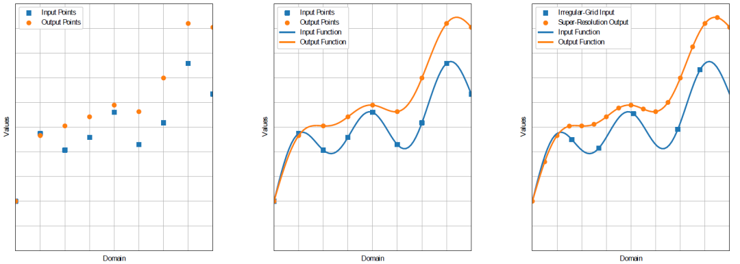

Figure 1 a, Neural networks learn the mapping between input and output points on fixed grids and discrete grids. b, Neural operators map functions between continuous domains, even when the training data is on fixed grids. c, Because neural operators map between functions, they accept inputs outside the training grid and can perform super-resolution processing. | Image source: Original Figure 2

2. Basic Architecture and Types of Neural Operators

2.1 Basic ArchitectureNeural operators have a structure similar to standard neural networks and can be divided into linear and nonlinear parts. As mentioned earlier, standard neural networks can only input and output data with fixed resolutions because they typically consist of a series of linear function modules, such as fully connected or convolutional layers, followed by nonlinear activation functions like Rectified Linear Units (ReLU). Standard neural networks resemble a spread-out spider web, where each node is a simple parameter. The basic architecture of neural operators is similar, with a linear module followed by nonlinear transformations, but the difference is that the linear part in neural operators computes integral operators rather than fixed-dimensional linear functions, such as the linear PDE solvers implemented by Green’s function integrals; it’s like each node of the spider web being drenched in dew, refracting the infinite details of the silk threads in the sunlight.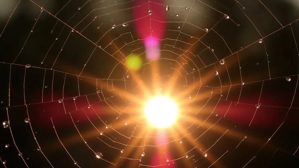

Figure 2 Demonstrating the potential of neural operators in handling tasks with infinite resolution data through the metaphor of a spider web drenched in dew | Image source: Stable Diffusion3 generation

Here is the expression for linear integral operators:

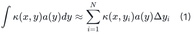
Where a( ⋅ ) is the input function of the operator block, and κ(x,y) represents the learnable kernel between any two points x and y in the output and input domains. In the linear integral operator, the output of the equation is not limited to the discreteness of the training data; it can be any point in the continuous domain (Figure 3a). For the input, the smaller the discreteness, the more accurate the approximation will be. The grid is a design that discretizes the solution domain in numerical computations, and neural operators have the property known as discretization convergence, meaning that as the input grid size approaches zero, the neural operator can converge to a unique operator (Figure 3b). This feature arises from the integral approximation methods used in neural operators, such as Riemannian sums, Galerkin spectral methods, or Fourier spectral methods. This is a key feature necessary for assessing the reliability of any scientific computation.After the linear integral operator, there is a pointwise nonlinear activation module, such as Gaussian Error Linear Units (GeLU). It is important to note that neural operators do not use ReLU because they are not smooth.2.2 Specific TypesBased on the parameterization methods of the integral operation in equation (1), there are many different architectures of neural operators. For example:1. DeepONet ModelThe DeepONet model is based on existing numerical methods and restricts the kernel κ(x,y) in equation (1) to the case where x and y are separable (i.e., κ(x,y)= κ₁(x) κ₂(y)). Although the initial DeepONet model was limited to fixed input grids, later extensions of DeepONet removed this restriction while retaining discretization convergence, making it a special case of neural operators.2. Graph Neural Operators (GNO)Graph Neural Operators (GNO) are operator extensions of graph neural networks that support kernel integration on fixed-radius spheres. Graph neural operators excel at tasks such as graph classification and link prediction, but their ability to capture global properties is limited. When the true operator is non-local, GNO may struggle to express global effects due to its limited receptive field if the radius is small. Increasing the receptive field and radius can make GNO computationally expensive. To address this issue, other global neural operators have been proposed.3. Fourier Neural Operators (FNO)Fourier Neural Operators (FNO) are another way to obtain global operators. FNO implements a series of layers that compute global convolution operators through Fast Fourier Transform (FFT), then mixes weights in the frequency domain and performs inverse Fourier transforms. By using learned coefficients in the Fourier domain (frequency domain) for element-wise multiplication (corresponding to convolution in the time domain), FNO can compute kernel integrals in equation (1) by returning to the original domain (time domain) through inverse Fourier transforms. By combining global convolution operators and nonlinear activations, FNO can approximate highly nonlinear and non-local solution operators. FNO and its variants can simulate many partial differential equations, such as the Navier-Stokes equations and seismic waves, perform high-resolution weather forecasting, and predict carbon dioxide migration with unprecedented cost and accuracy trade-offs. FNO methods are inspired by pseudo-spectral solvers that use Fourier bases and iteratively perform operations. Despite being inspired by this method, the nonlinear components of FNO give them greater expressive power. When handling regular grids, FNO demonstrates computational advantages due to its reliance on FFT. However, its limitations become apparent when handling irregular grids. Since FFT is only applicable to uniform grids, FNO requires interpolation or other deformation operations when dealing with non-uniform or irregular grids, which increases computational complexity and may introduce significant interpolation errors. To address this issue, some studies have proposed methods to convert irregular grids into regular grids, such as through deformation or graph kernel functions. Additionally, some research attempts to handle irregular geometries using geometric-aware Fourier transforms (such as Geo-FNO), which map physical space to regular computational space through deformation, allowing FFT to be applied on regular grids. However, these methods often require extensive data training and still face limitations when dealing with highly complex geometric shapes. In summary, FNO’s efficiency on regular grids is a significant advantage, but its scalability and computational efficiency are limited when handling irregular grids, necessitating further research and improvements to enhance its applicability in practical applications.4. Physics-Informed Neural Operators (PINO)In the early applications of neural networks, representing continuous functions with neural networks was an important proposition. For example, in graphics and scene processing, the use of continuous functions allows computers to achieve continuous visuals rather than a mosaic of individual pixels. This is known as implicit neural representation. The solution function of a single partial differential equation (PDE) represented by neural networks is called Physics-Informed Neural Network (PINN). For instance, in computer vision and graphics, implicit neural networks are used to represent a single velocity field or 3D scene. PINN and its variants have shown effectiveness in solving steady-state PDEs. However, optimizing PINN for time-varying PDEs is quite challenging, and standard gradient-based methods cannot easily yield solutions. Physics-Informed Neural Operators (PINO) have emerged to address this. In addition to PDE information, PINO combines training data, making the optimization landscape easier to handle and enabling learning of complex time-varying PDE solution operators. Furthermore, compared to purely data-driven neural operators, PINO demonstrates superior generalization and extrapolation capabilities, reducing the demand for training data by combining low-resolution training data with high-resolution physical constraints to achieve better approximations of underlying operators, enabling precise zero-shot super-resolution. Additionally, after training with other operators, PINO can further improve accuracy during testing by fine-tuning the model to minimize the PDE loss function. This fine-tuning step is similar to the PINN optimization process, but differs in that it initializes with a pre-trained PINO model and then fine-tunes it, rather than optimizing from a random initialization as in PINN. Thus, it can overcome the optimization difficulties present in PINN.5. Generative Neural OperatorsThe neural operators mentioned above are all used for deterministic mappings between approximate function spaces, but there is also a class of generative neural operators that extend deterministic mappings to probabilistic mappings over function spaces. The fundamental principle of these operators is to extend generative adversarial networks, diffusion models, or variational autoencoders to function spaces. Notably, diffusion neural operators take a Gaussian random field as input and can generate samples at any specified resolution. Generative neural operators have been applied to many scientific problems to fill in data for real-world phenomena that are difficult to obtain. This includes characteristics of input parameters for volcanic and seismic activity, as well as resolution-free visual sensors.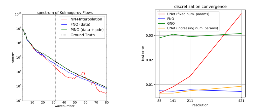

Figure 3 Examples of neural operators (using FNO and PINO) demonstrating advantages in output resolution (a) and the property of discretization convergence (b). a, x-axis is Fourier wave number, y-axis is the energy of each spectrum. Using the Kolmogorov flow for computing fluid motion as an example, Fourier Neural Operators (FNO) can extrapolate to unseen frequencies using only limited resolution training data. The low frequencies to the left of the vertical dashed line are training frequency resolutions, while the model extrapolates to higher frequencies to the right of the dashed line. Physics-Informed Neural Operators (PINO) simultaneously use training data and partial differential equations (PDEs) as loss functions and can perfectly recover the true frequency spectrum. The trained UNet (a popular neural network) combined with trilinear interpolation (NN + interpolation) exhibits severe distortion at higher frequencies beyond the training data resolution.

b, Neural operators exhibit discretization convergence, meaning that as discretization is refined, the model converges to the target continuous operator. x-axis is the resolution of the test data, y-axis is the test error at that given resolution. Here, the Darcy equation for calculating fluid motion in porous media is used as an example. Each architecture—UNet, FNO, and Graph Neural Operators (GNO)—is trained at a given resolution and tested at the same resolution (without super-resolution). As the resolution increases, FNO and GNO show consistent errors, but UNet’s error increases because its receptive field size varies with resolution. This demonstrates the advantage of neural operators over ordinary neural networks in terms of discretization convergence. | Image source: Original Figure 1

3. Applications of Neural Operators

Neural operators have shown significant advantages in multiple fields, such as:

1. Weather Forecasting: Neural operators are thousands of times faster than current numerical weather models in medium-range weather forecasting and have achieved accurate high-resolution (0.25 degrees) weather forecasting for the first time. This speedup makes risk assessments of extreme weather events (such as hurricanes and heatwaves) more accurate, as these events require multiple runs of weather models for uncertainty quantification.

2. Carbon Capture and Storage: In carbon capture and storage (CCS) applications, nested Fourier Neural Operator (FNO) models are hundreds of thousands of times faster than current numerical simulators, making large-scale assessments of geological CO₂ storage possible. This acceleration allows for probability assessments of maximum pressure accumulation and carbon dioxide plume footprints to be completed in just 2.8 seconds, while simulators would take nearly 2 years.

3. Solving Inverse Problems: In inverse problems or computer-aided design, it is often necessary to optimize a given set of parameters under a forward model to guide iterative design improvements or generate optimized designs from scratch. In practical applications, using neural operator models can produce optimized solutions for new medical catheter designs, reducing bacterial contamination by two orders of magnitude. Neural operator models can accurately simulate bacterial density in fluids flowing through pipes of arbitrary shapes, allowing for the optimization of catheter designs to prevent bacteria from entering the human body upstream.

4. Learning Long-Term Statistical Properties of Dynamic Systems: Neural operators have been used to learn attractors of chaotic systems and detect critical points in non-stationary systems. Neural operators based on generative adversarial networks or diffusion models in function spaces can be used to simulate stochastic natural phenomena (such as volcanic and climatic activities) and stochastic differential equations.

5. Other Applications: Neural operators have also been used in fluid dynamics, 3D industrial-grade automotive aerodynamics, urban microclimate modeling, material deformation, computational lithography, photoacoustic imaging, and electromagnetic field simulations.

4. Summary and Outlook

Neural operators aim to learn the solution operators of partial differential equations in a grid-convergent manner. Compared to standard neural networks, neural operators are more suitable for solving partial differential equations. Neural operators can learn directly from observational data without being affected by modeling errors in numerical methods. When used for inverse problems, such as optimizing design generation, they exhibit a level of innovation similar to that of general researchers. The application of neural operators can also simplify and lower the significant cross-disciplinary barriers and learning costs of modern scientific research and industry, as running well-trained neural operators does not require the deep domain expertise needed by traditional solvers. Of course, as a modern deep learning model, neural operators also face overfitting issues. In settings with minimal data, they may overfit the training data; in very low-resolution scenarios, they may overfit the lack of resolution. In these cases, they may lack the generalization ability to handle out-of-distribution data beyond the average. These issues can be addressed through the integration of domain knowledge in design, more data, higher fidelity data, and physical equations. The fundamental properties of neural operators tell us good news—that AI cannot take away most scientists’ jobs in the short term, as the reliability of all results still relies on human judgment. However, the authors of this article believe that neural operators provide a transformative approach for data simulation and process design, enabling rapid research and development. AI may not yet dominate scientific research, but perhaps this is due to our lack of a “scientific method dataset.” Neural operators embody the powerful computational capability of obtaining continuous functions, and perhaps in the near future, we will experience their role in accelerating human cognition of the material world.References[1]Z. Li et al., “Fourier Neural Operator for Parametric Partial Differential Equations,” arXiv:2010.08895 [cs, math], Oct. 2020, Available: arXiv:2010.08895v3[2]Li, Zongyi, et al. “Fourier Neural Operator with Learned Deformations for PDEs on General Geometries.” ArXiv.org, 11 July 2022, arxiv.org/abs/2207.05209.[3]T. Kurth, “FourCastNet: Accelerating Global High-Resolution Weather Forecasting Using Adaptive Fourier Neural Operators”, 2023, pp. 1–11. doi: 10.1145/3592979.3593412.[4]G. Wen, Z. Li, Q. Long, Kamyar Azizzadenesheli, Anima Anandkumar, and S. Benson, “Real-time high-resolution CO(2) geological storage prediction using nested Fourier neural operators,” Energy & Environmental Science, vol. 16, no. 4, pp. 1732–1741, Jan. 2023, doi: 10.1039/d2ee04204e.[5]H. Sun, Y. Yang, K. Azizzadenesheli, R. W. Clayton, and Z. E. Ross, “Accelerating Time-Reversal Imaging with Neural Operators for Real-time Earthquake Locations,” arXiv:2210.06636 [physics], Oct. 2022, Available: arXiv:2210.06636v1[6]T. Zhou et al., “AI-aided geometric design of anti-infection catheters,” Science Advances, vol. 10, no. 1, Jan. 2024, doi: 10.1126/sciadv.adj1741.

AI+Science Reading Club

AI+Science is a trend that has emerged in recent years, combining artificial intelligence and science. On one hand is AI for Science, where machine learning and other AI technologies can be used to solve problems in scientific research, from predicting weather and protein structures to simulating galaxy collisions, optimizing nuclear fusion reactor designs, and even conducting scientific discoveries like scientists, referred to as the “fifth paradigm” of scientific discovery. On the other hand is Science for AI, where laws and ideas in science, especially in physics, inspire machine learning theory, providing new perspectives and methods for the development of artificial intelligence.The Wisdom Club, in collaboration with postdoctoral researcher Wu Tailin from Stanford University’s Department of Computer Science (under Professor Jure Leskovec), Harvard Quantum Initiative researcher He Hongye, and MIT Physics PhD student Liu Ziming (under Professor Max Tegmark), jointly initiated a reading club themed “AI+Science” to explore important issues in this field and collaboratively study related literature. The reading club has concluded, but you can now join the community and unlock access to replay videos.

For more details, see: A New Paradigm of Mutual Empowerment Between Artificial Intelligence and Scientific Discovery: Launch of the AI+Science Reading ClubRecommended Reading1. Fourier Neural Operators: Applications of Fourier Transform in Deep Learning to Solve Partial Differential Equations2. Frontier Progress: Koopman Neural Operators for Solving Partial Differential Equations3. How to Discover the Next AlphaFold and ChatGPT in AI+Science?4. Zhang Jiang: The Foundation of Third-Generation Artificial Intelligence Technology—From Differentiable Programming to Causal Inference | New Course from Wisdom Academy5. As the Year of the Dragon Begins, It’s a Great Time to Learn! Unlock All Content from Wisdom Academy and Start Your New Year Learning Plan

6. Join Wisdom Academy, Let’s Explore Together!

Click “Read Original” to sign up for the reading club