This article shares an analysis of the mathematical principles behind CNNs, which will help you deepen your understanding of how neural networks work in CNNs. As a suggestion, this article will include quite complex mathematical equations. If you’re not accustomed to linear algebra and calculus, that’s fine; the goal is not to memorize these formulas but to have an intuitive understanding of what happens below.Complete source code with visualizations and annotations:GitHub: https://github.com/SkalskiP/ILearnDeepLearning.py
Introduction
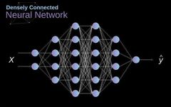
In the past, we have learned about these densely connected neural networks. The neurons in these networks are divided into several groups, forming continuous layers. Each such neuron is connected to every neuron in the adjacent layer. The figure below shows an example of this architecture.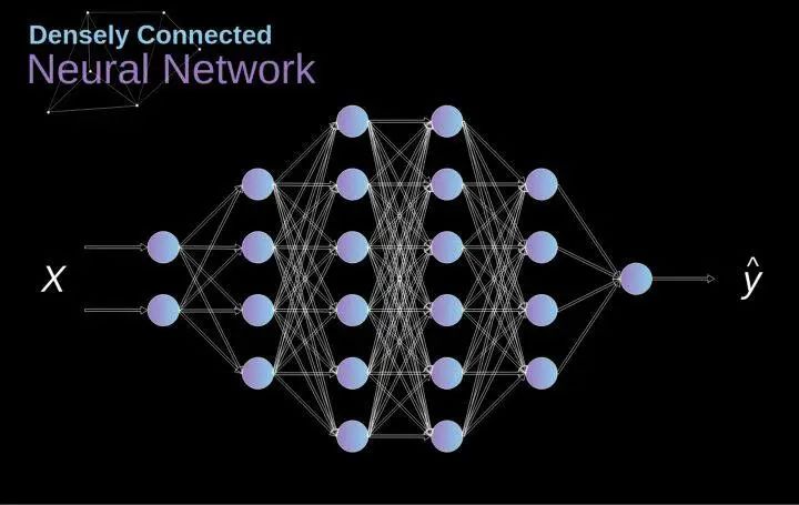 Figure 1. Structure of a densely connected neural network When we solve classification problems based on a finite set of artificially designed features, this method is very effective. For example, we can predict a football player’s position based on their statistics during a match. However, when dealing with photos, the situation becomes much more complicated. Of course, we can treat each pixel’s value as a separate feature and pass it as input to our dense network.Unfortunately, to make this network suitable for a specific smartphone photo, it must contain tens of millions or even billions of neurons. On the other hand, we could downscale our photos, but in the process, we would lose some useful information.We immediately realize that traditional strategies do not work for us; we need a new effective method to leverage as much data as possible while reducing the necessary computation and parameter count. This is where CNNs come into play. Data Structure of Digital Images Let’s take some time to explain how digital images are stored. Most of you may know that they are actually composed of many numbers arranged in a matrix. Each such number corresponds to the brightness of a pixel. In the RGB model, a color image is actually composed of three matrices corresponding to the red, green, and blue color channels.In black-and-white images, we only need one matrix. Each matrix stores values between 0 and 255. This range is a compromise between the efficiency of storing image information (values within 256 can be expressed in a single byte) and the sensitivity of the human eye (we can distinguish a limited number of the same color grayscale values).
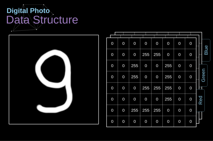 Figure 2. Data structure of digital images Convolution kernels are not only used in neural networks but are also a key part of many other computer vision algorithms. In this process, we take a smaller matrix (called a kernel or filter), input the image, and transform the image based on the values of the filter. The resulting feature map values are calculated using the following formula, where the input image is represented by f, our kernel is represented by h, and the row and column indices of the resulting matrix are represented by m and n, respectively.
 Figure 3. Example of kernel convolution After placing the filter on the selected pixel, we extract the corresponding values from the kernel and multiply them pairwise with the corresponding values in the image. Finally, we sum everything up and place the result in the corresponding position of the output feature map.Above, we can see how such an operation is implemented in detail, but what is more concerning is what applications can be achieved by performing kernel convolution on a complete image. Figure 4 shows the convolution results of several different filters.
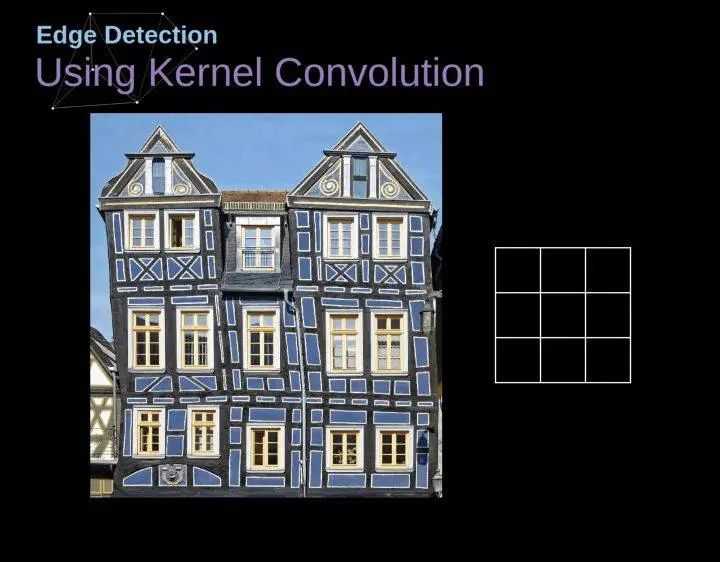 Figure 4. Edge detection through kernel convolution [Original image: https://www.maxpixel.net/Idstein-Historic-Center-Truss-Facade-Germany-3748512]
Valid Convolution and Same Convolution
As shown in Figure 3, when we convolve a 6×6 image with a 3×3 kernel, we obtain a 4×4 feature map. This is because there are only 16 different positions where we can place the filter in this image. Each convolution operation reduces the size of the image, so we can only perform a limited number of convolutions until the image disappears completely.More importantly, if we observe how the convolution kernel moves through the image, we will find that the influence of pixels located at the edges of the image is much smaller than that of pixels located in the center of the image. Thus, we lose some information contained in the image. The following figure shows how the position of a pixel changes its influence on the feature map. Figure 5. The influence of pixel position To solve these two problems, we can pad the image with an extra border. For example, if we use 1px padding, we increase the size of the photo to 8×8, and then the output of convolving with a 3×3 filter will be 6×6. In practice, we generally use 0 to pad the extra padding area. Depending on whether we use padding, we determine between two types of convolutions – valid convolution and same convolution.This naming is not very appropriate, so for clarity: Valid means we only use the original image, Same means we also consider the surrounding borders of the original image, so the input and output image sizes are the same. In the second case, the padding width should satisfy the following equation, where p is the padding width and f is the filter dimension (generally odd).
Stride Convolution
 Figure 6. Example of stride convolution In the previous examples, we always moved the convolution kernel one pixel at a time. However, the stride can also be viewed as one of the hyperparameters of the convolution layer. In Figure 6, we can see what the convolution looks like if we use a larger stride.When designing a CNN architecture, if we want less overlapping of the receptive fields or want a smaller spatial dimension of the feature map, we can decide to increase the stride. The size of the output matrix – considering the padding width and stride – can be calculated using the following formula.
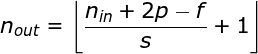
Transition to Three Dimensions
Spatial convolution is a very important concept that allows us not only to process color images but also to apply multiple convolution kernels in a single layer. The first important principle is that the filter and the image to which it is applied must have the same number of channels. Basically, this method is very similar to the example in Figure 3, but this time we will multiply the values in three-dimensional space with the corresponding convolution kernel.If we want to use multiple filters on the same image, we convolve them separately, stack the results together, and combine them into a whole. The dimensions of the receiving tensor (i.e., our three-dimensional matrix) satisfy the following equation: n – image size, f – filter size, nc – number of channels in the image, p – whether padding is used, s – stride used, nf – number of filters. 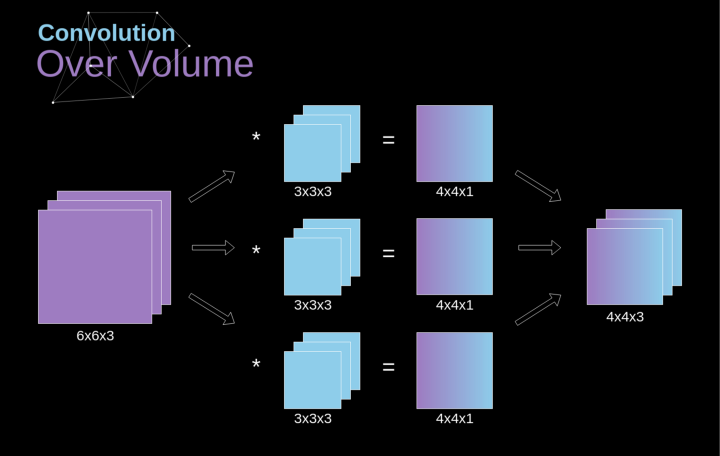
 Figure 7. Three-dimensional convolution
Convolution Layer
Now it’s time to apply the knowledge we’ve learned today to construct our CNN layer.Our approach is almost the same as the one we used in densely connected neural networks, the only difference being that this time we will use convolution instead of simple matrix multiplication.Forward propagation involves two steps.The first step is to calculate the intermediate value Z, which is the result of the convolution obtained using the input data and the weight tensor W from the previous layer (including all filters), then adding the bias b.The second step is to apply a nonlinear activation function to the obtained intermediate value (our activation function is represented as g). Interested readers regarding the matrix equation can find the corresponding mathematical formula below. By the way, in the following figure, you can see a simple visualization describing the dimensions of the tensors used in the equation.  Figure 8. Tensor dimensions
Connection Pruning and Parameter Sharing
At the beginning of the article, I mentioned that densely connected neural networks are not good at processing images because they require learning a large number of parameters. Now that we understand what convolution is, let’s consider how it optimizes computation.In the figure below, the two-dimensional convolution is shown in a slightly different way, with the neurons marked with numbers 1-9 forming the input layer and accepting the pixel brightness values of the image, while units A – D represent the computed feature map elements. Finally, I-IV are the values of the convolution kernels that need to be learned. Figure 9. Connection pruning and parameter sharingNow, let’s focus on two very important properties of convolution layers.First, you can see that not all neurons in consecutive layers are interconnected. For example, neuron 1 only affects the value of A.Secondly, we see that some neurons share the same weights. These two properties mean that the number of parameters we need to learn is much less.By the way, it is worth noting that a value in the filter affects every element in the feature map – this is very important in the backpropagation process. Backpropagation in Convolution LayersAnyone who has ever tried to write their own neural network code from scratch knows that completing forward propagation is only half of the entire algorithm process. The real fun begins when you want to perform backpropagation. Now, we don’t need to be troubled by this backpropagation issue; we can leverage deep learning frameworks to implement this part, but I think it’s valuable to understand the underlying principles. Just like in densely connected neural networks, our goal is to compute the derivatives and then use them to update our parameter values, a process called gradient descent.In our calculations, we need to use the chain rule – I mentioned it in previous articles. We want to evaluate how changes in parameters affect the final feature map and subsequently the final result. Before we begin discussing the details, let’s unify the mathematical notation used – to simplify the process, I will abandon the complete notation of partial derivatives and use the shorter notation as shown below. But remember, when I use this notation, I always refer to the partial derivative of the loss function.
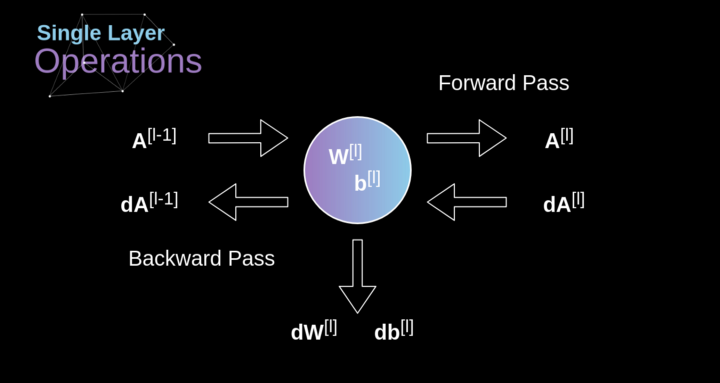 Figure 10. Forward and backward propagation of a single convolution layer’s input and output Our task is to compute dW[l] and db[l] – which are the derivatives related to the parameters of the current layer, as well as the value of dA[l -1] – which will be passed to the previous layer. As shown in Figure 10, we receive dA[l] as input. Of course, the dimensions of the tensors dW and W, db and b, and dA and A are the same. The first step is to obtain the intermediate value dZ[l] by taking the derivative of the activation function of the input tensor. According to the chain rule, the results obtained from this operation will be used later.
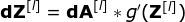 Now, we need to deal with the backpropagation of the convolution itself. To achieve this, we will use a matrix operation called full convolution, as shown in the figure below. Note that in this process, we rotate the convolution kernel 180 degrees before using it. This operation can be described by the following formula, where the filter is represented by W, and dZ[m,n] is a scalar belonging to the partial derivative of the previous layer.
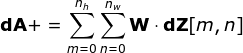
 Figure 11. Full convolution Pooling LayerIn addition to convolution layers, CNNs also frequently use what is known as a pooling layer. Pooling layers are primarily used to reduce the size of tensors and accelerate computation. This type of network layer is simple – we need to divide the image into different regions and then perform some operations on each part.For example, in a max pooling layer, we select the maximum value from each region and place it in the corresponding position in the output. In the case of convolution layers, we have two hyperparameters – filter size and stride. One last important point is that if we are to perform pooling operations on multi-channel images, we should perform pooling separately for each channel.
  Figure 12. Example of max pooling Backpropagation in Pooling LayersIn this article, we will only discuss the backpropagation of max pooling, but the rules we learn can be easily adjusted to apply to all types of pooling layers. Since there are no parameters to update in this type of layer, our task is simply to distribute the gradients appropriately.As we remember, in the forward propagation of max pooling, we select the maximum value from each region and pass them to the next layer.Therefore, it is clear that during backpropagation, the gradients should not affect the elements in the matrix that were not included in the forward propagation.In fact, this is achieved by creating a mask that remembers the positions of the values used in the first stage, which we can later use to propagate the gradients.
  Figure 13. Backpropagation of max pooling Reference: https://towardsdatascience.com/gentle-dive-into-math-behind-convolutional-neural-networks-79a07dd44cf9
Editor / Zhang Zhihong
Reviewer / Fan Ruiqiang
Verified by / Zhang Zhihong
Click below
Follow us
Read the original text