Summary of Convolutional Neural Network Compression Methods

Click on the above “Beginner Learning Vision”, choose to add Star Mark or Top.

Important content delivered at the first time

We know that to some extent, the deeper the network, the more parameters it has, and the more complex the model, the better its final effect. The neural network compression algorithm aims to convert a large and complex pre-trained model into a compact small model. According to the degree of damage to the network structure during the compression process, we divide model compression techniques into “frontend compression” and “backend compression”.

Frontend compression refers to compression techniques that do not change the original network structure, mainly including knowledge distillation, compact model structures, and pruning at the filter layer level.

Backend compression refers to techniques that include low-rank approximation, unrestricted pruning, parameter quantization, and binary networks, aiming to minimize model size and significantly alter the original network structure.

In summary: Frontend compression hardly changes the original network structure (it merely reduces the number of layers or filters based on the original model), while backend compression causes irreversible and significant changes to the network structure, leading to incompatibilities with existing deep learning frameworks and even hardware devices after such changes. Its maintenance cost is very high.

1. Low-Rank Approximation

Simply put, the weight matrix of convolutional neural networks is often dense and large, resulting in high computational overhead. One method is to use low-rank approximation techniques to reconstruct this dense matrix from several small-scale matrices, which is classified as a low-rank approximation algorithm.

Generally, the rank of a row echelon matrix equals its “step number”—the number of non-zero rows.

The principle of low-rank approximation algorithm in reducing computational overhead is as follows:

Given a weight matrix, if it can be represented as a combination of several low-rank matrices, i.e., where each low-rank matrix can be decomposed into a product of small-scale matrices, then when the rank is very small, it can significantly reduce overall storage and computational overhead.

Based on the above idea, Sindhwani et al. proposed an algorithm using structured matrices for low-rank decomposition, and the specific principle can be referred to in their paper. Another simpler method is to use matrix decomposition to reduce the parameters of the weight matrix, as proposed by Denton et al., using Singular Value Decomposition (SVD) to reconstruct the weights of fully connected layers.

1.1 Summary

The low-rank approximation algorithm has achieved good results on medium and small network models, but its hyperparameter amount shows a linear trend with the number of network layers. As the number of layers and model complexity increase, its search space will expand dramatically. Currently, it is mainly studied in academia, with few applications in industry.

2. Pruning and Sparse Constraints

Given a pre-trained network model, common pruning algorithms generally follow these operations:

1. Measure the importance of neurons.

2. Remove some unimportant neurons; this step is simpler and more flexible than the previous one.

3. Fine-tune the network. Pruning operations inevitably affect the network’s accuracy, and to prevent excessive damage to classification performance, the pruned model needs to be fine-tuned. For large-scale image datasets (such as ImageNet), fine-tuning can consume a lot of computational resources, so the extent of fine-tuning must be considered.

4. Return to the first step and repeat the next round of pruning.

Based on the above iterative pruning framework, different researchers have proposed various methods. Han et al. proposed first removing all weight connections below a certain threshold, then fine-tuning the pruned network to update parameters. The drawback of this method is that the pruned network is unstructured, meaning the removed network connections lack continuity in distribution, leading to frequent switching between CPU caches and memory, thus limiting actual acceleration effects.

Based on this method, some scholars have attempted to raise the granularity of pruning to the entire filter level, discarding entire filters. However, how to measure the importance of filters is a challenge. One strategy is to use statistical measures of filter weights, such as calculating the L1 or L2 values of each filter and using the corresponding values as standards for measuring importance.

Using sparse constraints for network pruning is also a research direction, where the idea is to add a sparsity regularization term for weights in the network’s optimization objective, causing some weights to approach 0 during training, and these 0 values become the targets for pruning.

2.1 Summary

Overall, pruning is an effective universal compression technique to reduce model complexity, with the key being how to measure the importance of individual weights to the overall model. The pruning operation causes minimal damage to the network structure, and combining pruning with other backend compression techniques can achieve maximum compression of the network model. Currently, there are cases in the industry using pruning methods for model compression.

3. Parameter Quantization

Compared to pruning operations, parameter quantization is a commonly used backend compression technique. The so-called “quantization” refers to deriving several “representatives” from the weights, which are used to represent specific values of a certain class of weights. The “representatives” are stored in a codebook, while the original weight matrix only needs to record the indices of their respective “representatives”, thus greatly reducing storage overhead. This idea can be likened to the classic bag-of-words model. Common quantization algorithms include:

1. Scalar quantization.

2. Scalar quantization can reduce network accuracy to some extent. To avoid this drawback, many algorithms consider structured vector methods, one of which is Product Quantization (PQ); details can be found in relevant papers.

3. Based on the PQ method, Wu et al. designed a universal network quantization algorithm: QCNN (Quantized CNN), whose main idea is that Wu et al. believe minimizing the reconstruction error of each layer’s network output is more effective than minimizing quantization error.

The basic idea of scalar quantization algorithms is to convert each weight matrix into vector form. Then, the elements of this weight vector are clustered into k clusters, which can be quickly completed using the classic k-means clustering algorithm:

Thus, only the k cluster centers and the scalar need to be stored in the codebook, while the original weight matrix only records the indices of their respective cluster centers in the codebook. If storage overhead of the codebook is not considered, this algorithm can reduce storage space to its original size. Scalar quantization based on k-means has proven very effective in many applications. The process of parameter quantization and codebook fine-tuning is shown below:

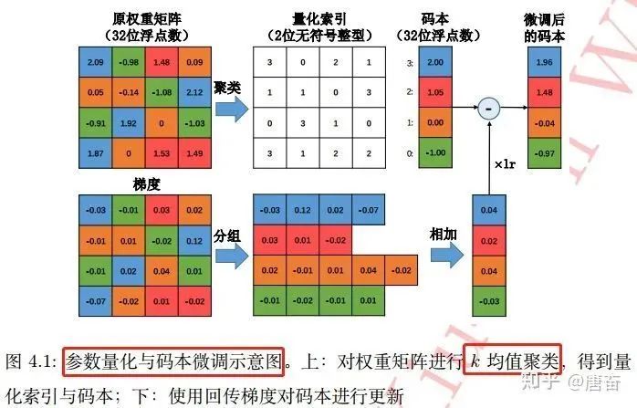
These three types of clustering-based parameter quantization algorithms fundamentally aim to map multiple weights to the same value, thereby achieving weight sharing and reducing storage overhead.

3.1 Summary

Parameter quantization is a commonly used backend compression technique that can significantly reduce model size with minimal performance loss. However, the drawback is that the quantized network is “fixed”, making it difficult to make any changes, and this method has poor universality, requiring specialized deep learning libraries to run the network.

4. Binary Networks

1. Binary networks can be seen as an extreme case of quantization methods: all weight parameters can only take values of +1 or -1, using 1 bit to store weights and features. In ordinary neural networks, a parameter is represented by a single-precision floating-point number, and binarizing parameters can reduce storage overhead to 1/32 of the original.

2. Binary neural networks have gained particular attention and development in recent years due to their high model compression rates and advantages in computation speed during forward propagation, becoming a very popular research direction in neural network model research. However, the first paper to truly binarize both weight values and activation function values in neural networks was published by Courbariaux et al. in 2016, titled “BinaryNet: Training Deep Neural Networks with Weights and Activations Constrained to +1 or -1.” This paper first provided methods for binarizing networks and training binary neural networks.

3. A typical CNN module consists of a sequence of operations: Convolution (Conv) -> Batch Normalization (BNorm) -> Activation (Activ) -> Pooling (Pool). For binary neural networks, the designed module consists of operations: Batch Normalization -> Binary Activation (BinActiv) -> Binary Convolution (BinConv) -> Pooling (Pool). This approach ensures that after batch normalization, the input mean is 0, then binary activation is applied to ensure data is either 0 or 1, followed by binary convolution, which maximally reduces feature information loss. The definition of the binary residual network structure instance code is as follows:

def residual_unit(data, num_filter, stride, dim_match, num_bits=1):
    """Residual Block Definition
    """
    bnAct1 = bnn.BatchNorm(data=data, num_bits=num_bits)
    conv1 = bnn.Convolution(data=bnAct1, num_filter=num_filter, kernel=(3, 3), stride=stride, pad=(1, 1))
    convBn1 = bnn.BatchNorm(data=conv1, num_bits=num_bits)
    conv2 = bnn.Convolution(data=convBn1, num_filter=num_filter, kernel=(3, 3), stride=(1, 1), pad=(1, 1))
    if dim_match:
        shortcut = data
    else:
        shortcut = bnn.Convolution(data=bnAct1, num_filter=num_filter, kernel=(3, 3), stride=stride, pad=(1, 1))
    return conv2 + shortcut

4.1 Gradient Descent of Binary Networks

Current neural networks are almost all trained based on gradient descent algorithms, but the weights of binary networks can only be ±1, making it impossible to directly compute gradient information and update weights. To solve this problem, Courbariaux et al. proposed the Binary Connect algorithm, which combines single precision and binary methods to train binary neural networks. The process is as follows:

1. Initialize weights as floating-point.

2. Forward Pass:

   – Use a deterministic method (sign(x) function) to quantize weights to +1/-1, using 0 as the threshold.
   – Use the quantized weights (only +1/-1) to compute forward propagation, performing convolution operations (which essentially only involves addition) to obtain the output of the convolution layer.

3. Backward Pass: Update gradients to floating-point weights (based on the relaxed sign function, calculate corresponding gradient values, and update single-precision weights based on these gradients);Training ends: permanently convert weights to +1/-1 for inference use.

4.2 Two Issues

Binary network binarization needs to solve two problems: how to binarize weights and how to compute gradients for binary weights.

1. How to binarize weights? Weight binarization generally has two choices:

• Directly binarize based on the sign of weights: . The sign function is defined as follows:

• Perform random binarization, i.e., for each weight, take with a certain probability.

1. How to compute gradients for binary weights? The gradient of binary weights is 0, making parameter updates impossible. To solve this problem, the sign function needs to be relaxed, using to replace . When is within the range , the gradient value is 1; otherwise, the gradient is 0.

4.3 Improvement of Binary Connect Algorithm

The previous Binary Connect algorithm only binarized weights, but the intermediate output values of the network remained single precision. Thus, Rastegari et al. improved this by proposing an algorithm that uses a single precision diagonal matrix multiplied by a binary matrix to approximate the original matrix, enhancing the classification performance of binary networks and compensating for their precision weaknesses. This algorithm decomposes the original convolution operation into the following process:

Where is the input tensor of this layer, is a filter corresponding to this layer, and is the binary weight for this filter.

Here, Rastegari et al. believe that relying solely on binary operations makes it difficult to achieve results equivalent to single precision convolution elements, so they use a single precision scaling factor to scale the results of binary filter convolutions. The value of can be determined based on the optimization objective:

Thus, obtaining . The training process of the improved binary connect algorithm is roughly similar to the previous algorithm, with the difference that the gradient computation process also considers the impact of . The presence of this single precision scaling factor effectively reduces reconstruction errors and achieves accuracy comparable to Alex-Net on the ImageNet dataset for the first time. As shown in the figure below:

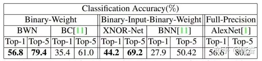
It can be seen that the accuracy of the weight binary neural network (BWN) is almost the same as that of the full precision neural network, but compared to the XOR neural network (XNOR-Net), there is a loss of over 10% in both Top-1 and Top-5 accuracy.

Compared to weight binary neural networks, XOR neural networks also convert the inputs of the network into binary values, so the multiplication and accumulation operations in XOR neural networks are replaced by bitwise XOR and popcount.

For more content, you can refer to these two articles:

https://github.com/Ewenwan/MVision/tree/master/CNN/Deep_Compression/quantization/BNN

https://blog.csdn.net/stdcoutzyx/article/details/50926174

4.4 Design Considerations for Binary Networks

• Avoid using Convolution with kernel = (1, 1) (including resnet bottlenecks): since all weights in binary networks are 1 bit, using a size of 1×1 will greatly reduce expressiveness.
• Increase the number of channels + increase the activation bit count should be coordinated: if you simply increase the number of channels, the feature map may waste model capacity due to low bit count. The reverse is also true.
• It is recommended to use 4 bits or fewer for activation bits; higher values yield diminishing precision returns but significantly increase inference computation.

5. Knowledge Distillation

This article only briefly introduces the pioneering work in this field – Distilling the Knowledge in a Neural Network, which is the “logits” distillation method; later papers also appeared on “features” distillation. For a deeper understanding, refer to this Chinese blog post – What is Knowledge Distillation? An Introductory Essay (https://zhuanlan.zhihu.com/p/90049906).

Knowledge distillation (https://arxiv.org/abs/1503.02531) is a form of transfer learning, simply put, it involves training a large model (teacher) and a small model (student), transferring the knowledge learned by the complex large model to the simplified small model through certain technical means, enabling the small model to achieve performance close to that of the large model.

In knowledge distillation experiments, we first train a teacher network, then use the output of the teacher’s network as the target for the student network, training the student network to ensure its results approach those of the teacher network, thus the loss function for the student network is . Here is the cross-entropy (Cross Entropy), is the one-hot encoding of the true label, is the output of the teacher network, and is the output of the student network.

However, directly using the softmax output from the teacher network may not be appropriate. After training, a network may have high confidence in the correct answer. For example, in the MNIST dataset, for an input of 2, the prediction probability for 2 is very high, while for similar digits like 3 and 7, the prediction probabilities are and . In this case, the teacher network’s learned similar information (e.g., digits 2 and 3, 7 are similar) is difficult to convey to the student network because their probabilities are close to 0. Therefore, the paper proposed the softmax-T (soft label calculation formula) as follows:

Here is the object the student network learns (soft targets), is the output logits before softmax of the teacher network. If is set to 1, the above formula becomes , calculating probabilities for each category based on the logits output. If approaches 0, the maximum value approaches 1 while other values approach 0, resembling one-hot encoding.

Thus, it can be seen that the final loss function of the student model consists of two parts:

• The first part consists of the cross-entropy between the predictions of the small model (student model) and the “soft labels” from the large model;

• The second part is the cross-entropy between the predictions of the small model and the ordinary category labels.

The importance of these two loss functions can be adjusted by certain weights. In practical applications, the value of T affects the final result; generally, a larger T can achieve higher accuracy. T (the distillation temperature parameter) is a type of hyperparameter in the training of knowledge distillation models. T is an adjustable hyperparameter; the larger the T, the softer the probability distribution (as described in the paper), and the curve becomes smoother, effectively adding perturbation during the transfer learning process, enhancing the student’s learning efficiency and generalization ability, which is essentially a strategy to mitigate overfitting. The entire process of knowledge distillation is shown in the figure below:

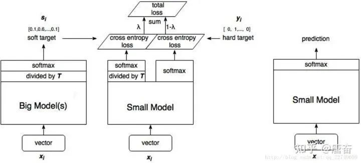
The actual model structure of the student model is the same as the small model, but the loss function includes two parts, with the knowledge distillation cross-entropy code example in MXNet as follows:

# -*-coding-*-  : utf-8  
"""
This program does not provide specific model structure code, mainly providing the softmax loss calculation part of knowledge distillation.
"""
import mxnet as mx

def get_symbol(data, class_labels, resnet_layer_num,Temperature,mimic_weight,num_classes=2):
    backbone = StudentBackbone(data)  # Backbone is the classification network backbone class
    flatten = mx.symbol.Flatten(data=conv1, name="flatten")
    fc_class_score_s = mx.symbol.FullyConnected(data=flatten, num_hidden=num_classes, name='fc_class_score')
    softmax1 = mx.symbol.SoftmaxOutput(data=fc_class_score_s, label=class_labels, name='softmax_hard')

    import symbol_resnet  # Teacher model
    fc_class_score_t = symbol_resnet.get_symbol(net_depth=resnet_layer_num, num_class=num_classes, data=data)

    s_input_for_softmax=fc_class_score_s/Temperature
    t_input_for_softmax=fc_class_score_t/Temperature

    t_soft_labels=mx.symbol.softmax(t_input_for_softmax, name='teacher_soft_labels')
    softmax2 = mx.symbol.SoftmaxOutput(data=s_input_for_softmax, label=t_soft_labels, name='softmax_soft',grad_scale=mimic_weight)
    group=mx.symbol.Group([softmax1,softmax2])
    group.save('group2-symbol.json')

    return group

TensorFlow code example is as follows:

# One-hot encode the category labels
one_hot = tf.one_hot(y, n_classes,1.0,0.0) # n_classes is the total number of categories, n is the category label
# one_hot = tf.cast(one_hot_int, tf.float32)
teacher_tau = tf.scalar_mul(1.0/args.tau, teacher) # teacher is the direct output tensor of the teacher model, tau is the temperature coefficient T
student_tau = tf.scalar_mul(1.0/args.tau, student) # The model directly outputs logits tensor student at temperature coefficient T
objective1 = tf.nn.sigmoid_cross_entropy_with_logits(student_tau, one_hot)
objective2 = tf.scalar_mul(0.5, tf.square(student_tau-teacher_tau))
"""
The final loss function of the student model consists of two parts:
The first part consists of the cross-entropy between the predictions of the small model and the soft labels from the large model;
The second part is the cross-entropy between predictions and ordinary category labels.
"""
tf_loss = (args.lamda*tf.reduce_sum(objective1) + (1-args.lamda)*tf.reduce_sum(objective2))/batch_size

tf.scalar_mul function is used to perform fixed multiplier scalar scaling on tf tensors. Generally, T values range from 1 to 20; here I referred to open-source code, and set it to 3. I found that in the open-source code, the training of the student model sometimes occurs along with the teacher model, while other times the student model is directly guided by the trained teacher model.

6. Shallow/Lightweight Networks

Shallow networks: Achieve approximation of complex model effects by designing a shallower (fewer layers) and more compact structure. However, the expressive ability of shallow networks is difficult to match that of deep networks. Therefore, the limitation of this design method is that it can only be applied to relatively simple problems, such as tasks with fewer categories in classification problems.

Lightweight networks: Using lightweight network structures such as MobilenetV2, ShuffleNetv2 as the model backbone can significantly reduce the number of model parameters.

References

1. https://www.cnblogs.com/dyl222/p/11079489.html
2. https://github.com/chengshengchan/model_compression/blob/master/teacher-student.py
3. https://github.com/dkozlov/awesome-knowledge-distillation
4. https://arxiv.org/abs/1603.05279
5. Analysis of Convolutional Neural Networks – Deep Learning Practice Handbook
6. https://zhuanlan.zhihu.com/p/81467832

Statement: Some content comes from the internet, for readers’ learning and communication purposes only. The copyright of the article belongs to the original author. If there are any issues, please contact for deletion.

Download 1: OpenCV-Contrib Extension Module Chinese Version Tutorial

Reply "OpenCV Extension Module Chinese Tutorial" in the backend of the "Beginner Learning Vision" public account to download the first Chinese version of the OpenCV extension module tutorial available online, covering over twenty chapters including extension module installation, SFM algorithms, stereo vision, object tracking, biological vision, super-resolution processing, etc.

Download 2: Python Vision Practical Projects 52 Lectures

Reply "Python Vision Practical Projects" in the backend of the "Beginner Learning Vision" public account to download 31 vision practical projects including image segmentation, mask detection, lane line detection, vehicle counting, eyeliner addition, license plate recognition, character recognition, emotion detection, text content extraction, facial recognition, etc., to assist in quickly learning computer vision.

Download 3: OpenCV Practical Projects 20 Lectures

Reply "OpenCV Practical Projects 20 Lectures" in the backend of the "Beginner Learning Vision" public account to download 20 practical projects based on OpenCV for advancing OpenCV learning.

Discussion Group

Welcome to join the reader group of the public account to communicate with peers. Currently, there are WeChat groups for SLAM, 3D vision, sensors, autonomous driving, computational photography, detection, segmentation, recognition, medical imaging, GAN, algorithm competitions, etc. (which will gradually be subdivided). Please scan the WeChat ID below to join the group, and note: "Nickname + School/Company + Research Direction", for example: "Zhang San + Shanghai Jiao Tong University + Vision SLAM". Please follow the format for notes; otherwise, it will not be accepted. After successful addition, you will be invited to related WeChat groups based on research direction. Please do not send advertisements in the group; otherwise, you will be removed. Thank you for your understanding~