
Source: Yunqi Community
This article contains 6500 words and is recommended to be read in 10 minutes. Starting from the historical development of neural networks, this article introduces the perceptron model, feedforward neural networks, and the BP algorithm.
[Introduction] What comes to mind when you think of neural networks? Have you ever pondered the principles behind deep learning? Since the birth of neural networks in the 1940s, it has undergone more than 70 years of development. What has happened during this time? This article will take you into the “past and present” of neural networks to explore.
Speaker Introduction:
Sun Fei (Dan Feng), Senior Algorithm Engineer of Alibaba Search Division. PhD from the Institute of Computing Technology, Chinese Academy of Sciences, with research focused on distributed text representation, having published multiple papers at SIGIR, ACL, EMNLP, and IJCAI. Currently engaged in research and development related to recommendation systems and text generation.
The following content is organized based on the speaker’s video sharing and PPT.
This session mainly revolves around the following five aspects:
-
The Development History of Neural Networks
-
The Perceptron Model
-
Feedforward Neural Networks
-
Backpropagation
-
Introduction to Deep Learning
1. The Development History of Neural Networks
Before introducing the history of neural networks, let’s first define what neural networks are. Neural networks refer to a simplified computational model designed to mimic the human brain, containing many neurons used for computation. These neurons are organized in a hierarchical manner through weighted connections, allowing for large-scale parallel computation and message passing between layers.
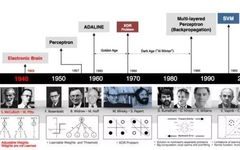
The following figure illustrates the entire development history of neural networks:
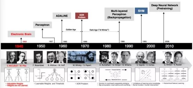
The development of neural networks predates the advent of computers, with the earliest neural network models appearing in the 1940s. This article will guide you through a basic understanding of neural networks based on their historical development.
The first generation of neuron models was verification-based, designed merely to validate that neuron models could perform computations. These models could neither be trained nor learn, and can be viewed as predefined logical gate circuits, with binary inputs and outputs and predefined weights.
The second era of neural networks occurred in the 1950s and 1960s, represented by works such as Rosenblatt’s perceptron model and Hebbian learning principle.
2. The Perceptron Model
The perceptron model is almost identical to the previously mentioned neuron model, but there are key differences. The activation function of the perceptron model can be a step function or a sigmoid function, and its input can be a real-valued vector instead of the binary vector of the neuron model. Unlike the neuron model, the perceptron model is a learnable model, with a notable feature being its geometric interpretation.
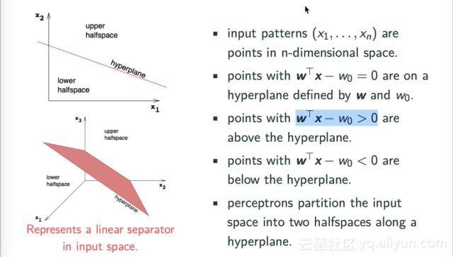
We can view the input values (x1, . . . , xn) as coordinates of a point in N-dimensional space, where w⊤x−w0 = 0 represents a hyperplane in N-dimensional space. Clearly, when w⊤x−w0 < 0, the point lies below the hyperplane, and when w⊤x−w0 > 0, it lies above. The perceptron model corresponds to a classifier’s hyperplane, which can separate different categories of points in N-dimensional space. As shown in the diagram below, the perceptron model is a linear classifier.
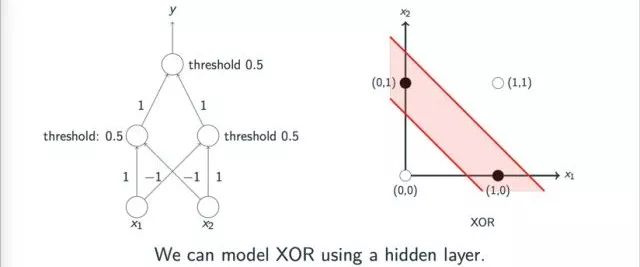
For basic logical operations like AND, OR, and NOT, the perceptron model can easily classify. However, can all logical operations be classified using a perceptron? The answer is no. For example, XOR operations are difficult to classify with a single linear perceptron, which is a major reason why neural network development quickly entered a low period after its first peak. This issue was first raised by Minsky et al. in their works on perceptrons, but there is a misconception about this work. In fact, Minsky et al. pointed out that XOR operations can be implemented through multi-layer perceptrons, but at the time, the academic community lacked effective learning methods to train multi-layer perceptron models, leading to the first low period in neural network development.
The intuitive geometric representation of multi-layer perceptrons implementing XOR operations is shown in the diagram below:

3. Feedforward Neural Networks
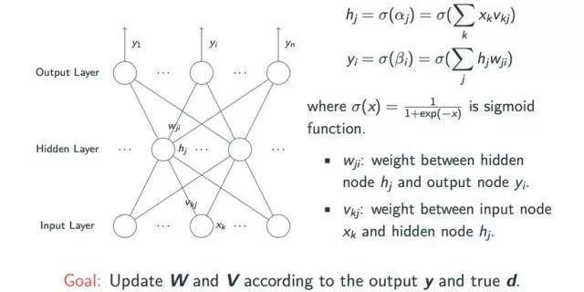
Entering the 1980s, due to the limited expressive power of single-layer perceptron neural networks, which could only perform linear classification tasks, the development of neural networks transitioned into the era of multi-layer perceptrons. A typical multi-layer neural network is the feedforward neural network, as shown in the diagram below, which includes input layers, hidden layers with variable node counts, and output layers. Any logical operation can be represented through multi-layer perceptron models, but this involves the weight learning problem among the three layers. The input layer nodes xk are multiplied by the weights vkj between the input layer and hidden layer, and then passed through an activation function such as sigmoid to obtain the corresponding hidden layer node value hj. Similarly, similar calculations can derive the output node value yi from hj.
The weights to be learned are the matrices w and v, and the final information obtained is the sample output y and the true output d. The specific process is shown in the diagram below:
If readers have a basic understanding of machine learning, they will know that typically, a model is learned based on the principle of gradient descent. In the perceptron model, applying the gradient descent principle is relatively straightforward. Taking the following diagram as an example, first, determine the model’s loss, which in this case uses squared loss, i.e., calculating the difference between the true output d and the model’s output y for convenience, typically adopting the squared relationship E = 1/2 (d−y)^2 = 1/2 (d−f(x))^2. According to the gradient descent principle, the weight update follows the rule: wj ← wi + α(d − f(x))f′(x)xi, where α is the learning rate that can be manually adjusted.
4. Backpropagation
For a multi-layer feedforward neural network, how do we learn all its parameters? First, the parameters at the top layer are easy to obtain, as we can derive parameter results based on the difference between the computed model output and the true output, using the gradient descent principle. However, the problem arises with hidden layers: although we can calculate their model output, we do not know their expected output, making it impossible to efficiently train a multi-layer neural network. This was a significant issue that troubled the academic community for a long time, leading to a lack of further development in neural networks after the 1960s.
Later, in the 1970s, many scientists independently proposed an algorithm called backpropagation. The basic idea of this algorithm is quite simple: although it was impossible to update the state of the hidden layers based on their expected output, it was possible to update the weights between the hidden layers and other layers based on the gradient of the error from the hidden layers. When calculating the gradient, since each hidden layer node is associated with multiple nodes in the output layer, it accumulates the errors from all previous layers.
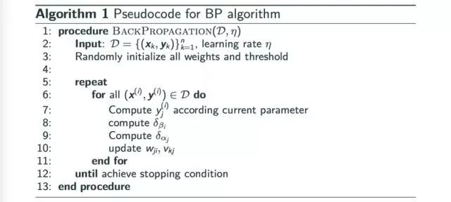
Another advantage of backpropagation is that the gradients and weight updates of nodes within the same layer can be computed in parallel, as they are not interrelated. The entire BP algorithm process can be represented in the following pseudocode:
Next, let’s introduce some other properties of BP neural networks. The BP algorithm is essentially a chain rule that can easily generalize to any directed graph computation. According to the gradient function, in most cases, BP neural networks yield only a local optimal solution, not a global optimal solution. However, generally speaking, the BP algorithm can compute a relatively good solution. The diagram below provides an intuitive demonstration of the BP algorithm:
In most cases, the BP neural network model will find a local minimum within a certain range, but by stepping outside this range, we may discover a better local minimum. In practical applications, there are many simple yet effective solutions to this issue, such as trying different random initialization methods. In fact, in today’s deep learning field, the initialization method has a significant impact on the final results. Another way to escape local minima during training is to introduce some random noise or use genetic algorithms to avoid the model getting stuck in undesirable local minima.
BP neural networks are an excellent model in machine learning, and when discussing machine learning, we must mention a fundamental problem frequently encountered throughout the process—overfitting. The common phenomenon of overfitting is that while the model’s loss continuously decreases on the training set, its loss and error on the test set may have already started to rise. There are two common ways to avoid overfitting:
-
Early Stopping: We can pre-define a validation set and run the model on this validation set while training, observing the model’s loss. If its loss on the validation set stops decreasing, we can stop the training even if the loss on the training set continues to decrease to prevent overfitting.
-
Regularization: We can add some regularization to the weights of the neural network edges. Recently, dropout—randomly dropping some nodes or edges—has become a common regularization method, which is also an effective way to prevent overfitting.
In the 1980s, neural networks were very popular, but unfortunately, in the 1990s, the development of neural networks fell into a second low period. There are many reasons for this decline, such as the rise of Support Vector Machines (SVM), which became a very popular model in the 1990s, making significant achievements across various applications and conferences. SVM has a well-established statistical learning theory, excellent intuitive explanations, high efficiency, and ideal results.
Consequently, the rise of statistical learning theories related to SVM somewhat suppressed the popularity of neural networks. On the other hand, from the perspective of neural networks themselves, although theoretically, BP can train networks of any depth, in practical applications, it becomes evident that the training difficulty of neural networks increases exponentially with the number of layers. For instance, in the early 1990s, it was already observed that in networks with many layers, phenomena such as gradient vanishing or gradient explosion could occur.
To illustrate gradient vanishing simply, suppose every layer of the neural network uses a sigmoid structure. During backpropagation, the loss will continuously form a gradient of sigmoid. If one of the gradients is very small, it will lead to increasingly smaller gradients as they propagate down. In fact, after propagating through just one or two layers, this gradient may have already vanished. Gradient vanishing results in deep parameters remaining almost static, making it difficult to derive meaningful parameter results. This is one reason why multi-layer neural networks are very challenging to train.
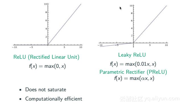
The academic community has conducted considerable research on this issue, with the simplest treatment being modifying the activation function. Early attempts involved using the Rectified activation function, as the sigmoid function, being exponential, is prone to gradient vanishing. Rectified replaces the sigmoid function with max(0,x), and as shown in the diagram below, for samples greater than 0, its gradient is 1, preventing gradient vanishing. However, when sample points are less than 0, its gradient becomes 0, indicating that ReLU is not a perfect solution. Subsequently, improved functions, including Leaky ReLU and Parametric Rectifier (PReLU), emerged, where when sample point x is less than 0, we can artificially multiply it by a coefficient such as 0.01 or α to prevent the gradient from becoming zero.
With the development of neural networks, subsequent methods have emerged to structurally address the difficulty of gradient propagation, such as meta-models, LSTM models, or the widely used cross-layer connections in image analysis to facilitate gradient propagation.
5. Introduction to Deep Learning
After the second low period of neural networks in the 1990s, by 2006, neural networks returned to public attention, and this resurgence was far more intense than any previous rise. A landmark event marking the resurgence of neural networks was the publication of two papers by Hinton et al. on multi-layer neural networks (now referred to as “deep learning”) in Salahudinov et al.’s work.
One paper addressed the previously mentioned issue of how to set initial values in neural network learning, proposing a straightforward approach: assuming the input value is x, the output is decoding x, thereby learning a better initialization point. The other paper proposed a method for rapidly training deep neural networks. The current popularity of neural networks can be attributed to many factors, including the substantial computational resources available today compared to earlier times, as well as the availability of large datasets. In the 1980s, the lack of substantial data and computational resources made it challenging to train large-scale neural networks.
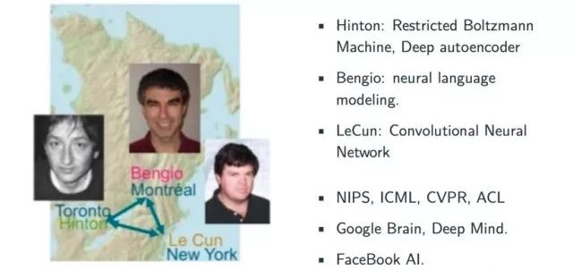
The early rise of neural networks is primarily attributed to three key figures: Hinton, Bengio, and LeCun. Hinton’s major contributions include Restricted Boltzmann Machines and Deep Autoencoders; Bengio’s significant achievements involve breakthroughs in meta-models applied to deep learning, which was one of the earliest fields to achieve practical breakthroughs; and LeCun’s notable work is in CNN research. The resurgence of deep learning is prominently reflected in major technical summits such as NIPS, ICML, CVPR, and ACL, with research departments like Google Brain, Deep Mind, and Facebook AI focusing their work on deep learning.

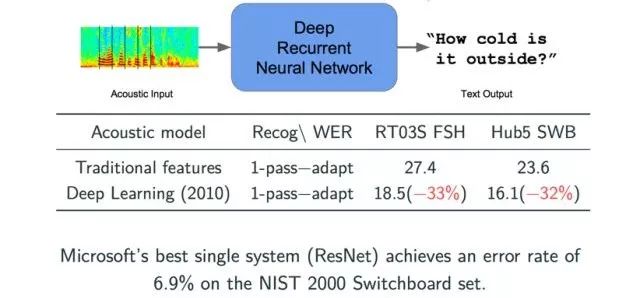
The first breakthrough after neural networks entered the public eye was in the speech recognition field. Before the application of deep learning theories, models were trained using predefined statistical libraries. In 2010, Microsoft employed deep learning neural networks for speech recognition, resulting in significant improvements in two error metrics, with nearly a one-third reduction in both metrics. Using the latest ResNet technology, Microsoft has reduced this metric to 6.9%, showing significant annual improvements.
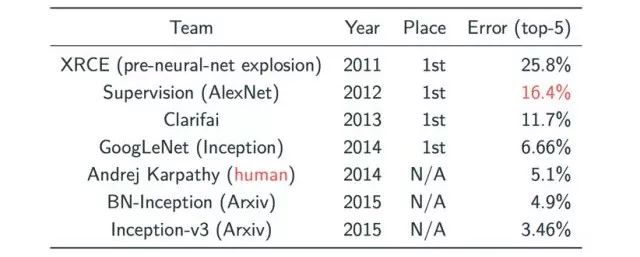
By 2012, in the image classification domain, CNN models achieved significant breakthroughs on ImageNet. Testing image classification involves a large dataset, requiring classification of these images into 1000 categories. Before the application of deep learning, the best result was an error rate of 25.8% (a result from 2011). After applying CNN to this image classification problem, Hinton and his students reduced this metric by nearly 10%. Since 2012, we have observed substantial annual breakthroughs in this metric, all achieved using CNN models.
The success of deep learning models can largely be attributed to their hierarchical structure, which enables them to learn autonomously and abstractly represent data through this structure. The abstracted features can be applied to various other tasks, which is one reason why deep learning is currently so popular.
Below are two very typical and commonly used deep learning neural networks: one is the Convolutional Neural Network (CNN) and the other is the Recurrent Neural Network (RNN).
1. Convolutional Neural Networks
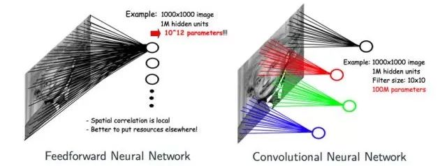
Convolutional Neural Networks have two core concepts: Convolution and Pooling. At this point, some may ask why we don’t simply use feedforward neural networks but instead adopt CNN models. For example, for a 1000×1000 image, a neural network would have 1,000,000 hidden layer nodes, and a feedforward neural network would need to learn on the order of 10^12 parameters, which is almost impossible due to the need for massive samples. However, for images, many parts share similar features. If we categorize images using CNN models based on the mathematical concept of convolution, each hidden layer node only connects to a local area of the image and scans its local features. Assuming each hidden layer node connects to a local sample size of 10×10, the final number of parameters would drop to 100M, and when multiple hidden layers share local parameters, the number of parameters decreases significantly.
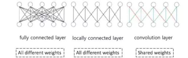
From the diagram below, we can intuitively see the differences between feedforward neural networks and CNNs. The models in the diagram move from left to right: a fully connected ordinary feedforward neural network, a locally connected feedforward neural network, and a convolution-based CNN model. We can observe that the connection weights between hidden layer nodes in convolution-based neural networks can be shared.
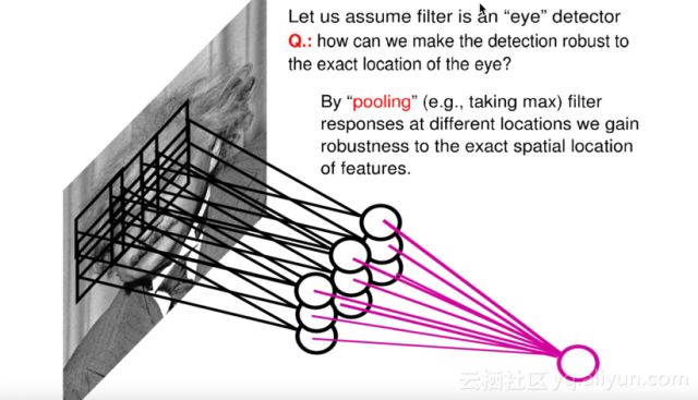
Another operation is Pooling. In addition to generating hidden layers through convolution, CNN will form an intermediate hidden layer—Pooling layer—where the most common pooling method is Max Pooling, which selects the maximum value from the obtained hidden layer nodes as output. Due to multiple kernels performing pooling, we obtain multiple intermediate hidden layer nodes. The benefits of this approach include: first, it further reduces the number of parameters; second, it possesses a certain degree of translation invariance. As shown in the diagram, if one of the nine hidden layer nodes shifts, the resultant pooling layer nodes remain unchanged.
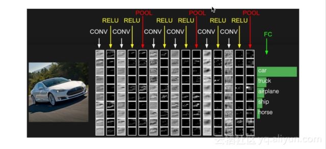
The two characteristics of CNN make it widely applicable in image processing, and it has even become a standard in image processing systems. The following visual example of a car illustrates CNN’s application in image classification. After inputting the original car image into the CNN model, starting from the most basic and rough features such as edges and points, through several convolutions and RELU activation layers, we can visually see that the features of the output image get closer to the outline of a car as we approach the top layer. This process ultimately yields a hidden representation that connects to a fully connected classification layer to derive the image’s category, such as car, truck, airplane, ship, horse, etc.
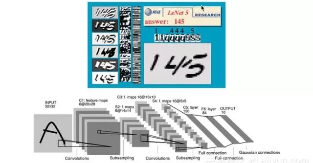
The following diagram illustrates an early neural network proposed by LeCun for handwritten recognition, which was successfully applied in the U.S. postal system in the 1990s. Interested readers can visit LeCun’s website to view the dynamic process of recognizing handwritten characters.
While CNNs are very popular in the image domain, in recent years, CNNs have also been extensively applied in the text domain. For instance, the current best model for text classification is based on CNN models. From the perspective of text classification, identifying a text’s category essentially involves recognizing some keyword signals within that text, a task well-suited for CNN models.
In fact, today’s CNN models have been applied across various fields in people’s lives, such as criminal investigation, the development of autonomous vehicles, segmentation, and Neural Style, among others. Neural Style is a fascinating application; for example, the popular App Store application Prisma allows users to transform uploaded photos into other styles, such as turning them into paintings resembling Van Gogh’s Starry Night, heavily utilizing CNN technology.
2. Recurrent Neural Networks
The basic principles of recurrent neural networks are illustrated in the diagram below. From the diagram, we can see that the output of a recurrent neural network depends not only on the input x but also on the current hidden state, which is updated based on the previous x. The advantage of recurrent neural network models lies in their suitability for handling sequential data such as text, language, or speech, where the current data state is influenced by previous data states. Feedforward neural networks struggle to achieve this.

When discussing RNNs, we must mention the previously addressed LSTM model. In fact, LSTM is not a complete neural network but rather a result of complex processing of nodes within an RNN. LSTM contains three gates: input gate, forget gate, and output gate.
These three gates handle the data content within the cell, determining whether to input, forget, or output the data content of the cell.

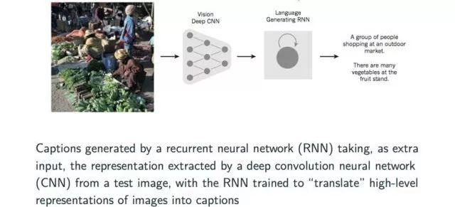
Finally, let’s introduce a currently popular cross-domain neural network application—converting an image into descriptive text or a title for that image. The implementation process can be simply explained as first extracting information from the image using a CNN model to form a vector representation, and then inputting that vector into a trained RNN model to derive the description of the image.
Live video review address: https://yq.aliyun.com/video/play/1370?spm=a2c41.11124528.0.0