

Author:Qiu Zhenyu (Algorithm Engineer, Huatai Securities Co., Ltd.)
Zhihu Column:My AI Journey
Recently, I came across a paper titled “Revisiting Few-sample BERT Fine-tuning”. The paper has just been released on arXiv, and although it hasn’t attracted much attention yet, I found it very practical after reading it, making it suitable for application in real business scenarios. This article mainly interprets and experimentally verifies some viewpoints from this paper.
Without further ado, let’s get straight to the point. The main theme of this paper is how to use BERT more effectively for fine-tuning on small datasets. The paper points out that the current fine-tuning of BERT is unstable, especially on small datasets. In the early stages of training, the model continues to oscillate, which reduces the efficiency of the entire training process, slows down the convergence speed, and also decreases the model’s accuracy to some extent. The article summarizes three optimization directions, discussing how to stabilize the fine-tuning of the BERT model on small datasets from the perspectives of optimization methods, weight parameters, and training methods. Below, I will interpret each of these three perspectives in detail.
Debiasing of Adam Optimization
I wonder if anyone has noticed that the Adam implementation in the official BERT source code for TensorFlow or PyTorch differs slightly from the original Adam implementation. Let’s briefly review the steps of the Adam algorithm:
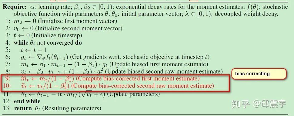
Adam mainly combines first-order momentum and second-order momentum moving averages, supplemented by adaptive changes in the learning rate, making model training more efficient and allowing for adaptive learning rate changes. In addition, there is an algorithm detail in Adam that needs attention, which is bias correction. Notice the part marked in red in the image above: before the gradient update operation, both first-order and second-order momentum need to be bias-corrected. The reason for this is that the momentum in Adam is initialized to 0. Therefore, in the early stages of model training and when the exponential decay rate hyperparameter ( ) is very small, the momentum estimate is easily biased towards 0, and at this point, we need to perform a bias correction on the momentum, as specifically illustrated in the red box in the image. The specific derivation can be referenced in the original Adam paper. Here, as an example, we will briefly review the derivation of the second-order momentum:
The main logic of the derivation is to establish the expectation of the second-order momentum  and the expression relationship of the expectation of
  .
.
First, according to step 8 in the image above, the second-order momentum  can be transformed into a function of the gradient
  at historical timestamps:

Taking the expectation of both sides yields:

(updated on 2020.06.17) New content: Here, I researched the derivation again and finally saw an answer on a website that made some sense. I am posting it here for your reference: Understanding a derivation of bias correction for the Adam optimizer.
First, we need to understand how  is obtained. It is speculated that
  estimates the error term of the historical gradient
  based on the current gradient
  . With this error term, we can take the
  term out of the summation formula and no longer depend on i. All terms containing
  can be considered constants at this point and can be taken out of the expected brackets. When the second-order momentum is a steady-state distribution, it is a constant at every time t, thus
  is 0.
is 0.
Next, another question is how to simplify  into
into  . This requires using the finite geometric series summation formula. For a finite geometric series, its summation can be expressed as follows:

Self-deprecating: I have forgotten all my high school math, feeling embarrassed…
At this point, substituting  into the above formula, and since we have already taken the current
  out of the summation formula, we can derive as follows:

The second term of the above equality can be obtained by multiplying  to the right-hand division term, while multiplying both the numerator and denominator by
  to get the third term.
Here,  can be made to approach 0 by controlling the decay rate hyperparameter
  . Thus, the remaining offset influencing factor is
  . Therefore, we achieve bias correction by dividing
  by this term.
This derivation is not very deep due to my limited mathematical ability, so I welcome students who are good at math to critique.
BERT’s Adam
We check the official BERT source code project provided by Google (github.com/google-resea) in its optimization.py file. In the AdamWeightDecay class, we can see that it omits the bias correction step mentioned above:
m = tf.get_variable(
          name=param_name + "/adam_m",
          shape=param.shape.as_list(),
          dtype=tf.float32,
          trainable=False,
          initializer=tf.zeros_initializer())
v = tf.get_variable(
          name=param_name + "/adam_v",
          shape=param.shape.as_list(),
          dtype=tf.float32,
          trainable=False,
          initializer=tf.zeros_initializer())

# Standard Adam update.
next_m = (
          tf.multiply(self.beta_1, m) + tf.multiply(1.0 - self.beta_1, grad))
next_v = (
          tf.multiply(self.beta_2, v) + tf.multiply(1.0 - self.beta_2,
                                                    tf.square(grad)))

update = next_m / (tf.sqrt(next_v) + self.epsilon)
By reviewing the original BERT paper, I found no specific explanation from the authors regarding this. It can only be speculated that when pre-training BERT, due to the large scale of training data and the high number of training steps, even without bias correction, the model can still gradually maintain stability during training, while reducing the computational cost of bias correction overall.
However, if this optimization method is still used in downstream tasks with fewer samples, it will lead to training instability. To verify this conclusion, the authors conducted detailed comparative experiments. They tried 50 different random seeds on four different datasets, using the original Adam with bias correction and the BERT Adam without correction for fine-tuning tasks. The experimental results verified the above viewpoints from different angles, as shown in the following figure:
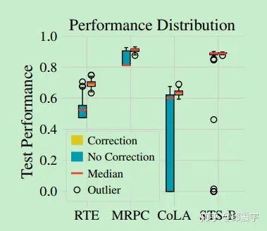
This is a box plot showing the test set performance of the model on different datasets, indicating that using bias-corrected Adam can significantly enhance the model’s performance on the test set across four datasets.
Next, let’s look at the following figure:
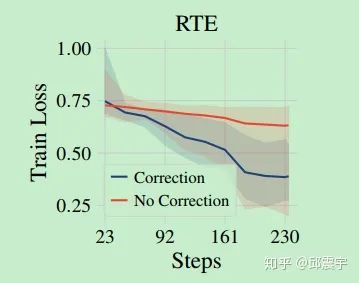
This figure reflects the training curve of the model on the small dataset RTE. It can be seen that using bias-corrected Adam for fine-tuning can achieve convergence faster while obtaining a lower loss.
Further Verification
Practice proves truth. To verify the effectiveness of the above conclusion, I decided to find a small dataset for actual testing. Recently, there was a named entity recognition competition held by CCKS, named the Named Entity Recognition Task for Experimental Identification. The training samples for this competition only total 400, with 4 entity types, which is indeed a small dataset, making it suitable for experimentation. The main model for the experiment is the BERT+CRF framework, with hyperparameters and random seeds kept constant, and the only variable being whether to use bias correction.
(updated on 2020.06.17) In the TensorFlow BERT implementation, to add the original bias correction, a certain amount of code needs to be added, mainly to increase the calculation and update of  and the logic calculation for bias correction. By reading the original TensorFlow Adam source code, it can be found that its bias correction is achieved by correcting the learning rate, that is,
  . In addition, TensorFlow also has its own computational graph optimization logic for updating and assigning
  , making it more complex compared to Keras code. Below is the code for AdamWeightDecay after adding the bias correction, which can be compared with the original Adam code:
class AdamWeightDecayOptimizer(optimizer.Optimizer):
    """A basic Adam optimizer that includes "correct" L2 weight decay."""

    def __init__(self,
                 learning_rate,
                 weight_decay_rate=0.0,
                 beta_1=0.9,
                 beta_2=0.999,
                 epsilon=1e-6,
                 exclude_from_weight_decay=None,
                 name="AdamWeightDecayOptimizer"):
        """Constructs a AdamWeightDecayOptimizer."""
        super(AdamWeightDecayOptimizer, self).__init__(False, name)

        self.learning_rate = learning_rate
        self.weight_decay_rate = weight_decay_rate
        self.beta_1 = beta_1
        self.beta_2 = beta_2
        self.epsilon = epsilon
        self.exclude_from_weight_decay = exclude_from_weight_decay
        self.learning_rate_t = None
        self._beta1_t = None
        self._beta2_t = None
        self._epsilon_t = None

    def _get_beta_accumulators(self):
        with ops.init_scope():
            if context.executing_eagerly():
                graph = None
            else:
                graph = ops.get_default_graph()
            return (self._get_non_slot_variable("beta1_power", graph=graph),
                    self._get_non_slot_variable("beta2_power", graph=graph))


    def _prepare(self):
        self.learning_rate_t = ops.convert_to_tensor(
            self.learning_rate, name='learning_rate')
        self.weight_decay_rate_t = ops.convert_to_tensor(
            self.weight_decay_rate, name='weight_decay_rate')
        self.beta_1_t = ops.convert_to_tensor(self.beta_1, name='beta_1')
        self.beta_2_t = ops.convert_to_tensor(self.beta_2, name='beta_2')
        self.epsilon_t = ops.convert_to_tensor(self.epsilon, name='epsilon')

    def _create_slots(self, var_list):
        first_var = min(var_list, key=lambda x: x.name)
        self._create_non_slot_variable(initial_value=self.beta_1,
                                    name="beta1_power",
                                    colocate_with=first_var)
        self._create_non_slot_variable(initial_value=self.beta_2,
                                    name="beta2_power",
                                    colocate_with=first_var)
        for v in var_list:
            self._zeros_slot(v, 'm', self._name)
            self._zeros_slot(v, 'v', self._name)

    def _apply_dense(self, grad, var):
        learning_rate_t = math_ops.cast(
            self.learning_rate_t, var.dtype.base_dtype)
        beta_1_t = math_ops.cast(self.beta_1_t, var.dtype.base_dtype)
        beta_2_t = math_ops.cast(self.beta_2_t, var.dtype.base_dtype)
        epsilon_t = math_ops.cast(self.epsilon_t, var.dtype.base_dtype)
        weight_decay_rate_t = math_ops.cast(
            self.weight_decay_rate_t, var.dtype.base_dtype)

        m = self.get_slot(var, 'm')
        v = self.get_slot(var, 'v')
        beta1_power, beta2_power = self._get_beta_accumulators()
        beta1_power = math_ops.cast(beta1_power, var.dtype.base_dtype)
        beta2_power = math_ops.cast(beta2_power, var.dtype.base_dtype)
        learning_rate_t = math_ops.cast(self.learning_rate_t, var.dtype.base_dtype)
        learning_rate_t = (learning_rate_t * math_ops.sqrt(1 - beta2_power) / (1 - beta1_power))

        # Standard Adam update.
        next_m = (
            tf.multiply(beta_1_t, m) +
            tf.multiply(1.0 - beta_1_t, grad))
        next_v = (
            tf.multiply(beta_2_t, v) + tf.multiply(1.0 - beta_2_t,
                                                   tf.square(grad)))

        update = next_m / (tf.sqrt(next_v) + epsilon_t)

        if self._do_use_weight_decay(var.name):
            update += weight_decay_rate_t * var

        update_with_lr = learning_rate_t * update

        next_param = var - update_with_lr

        return control_flow_ops.group(*[var.assign(next_param),
                                        m.assign(next_m),
                                        v.assign(next_v)])

    def _resource_apply_dense(self, grad, var):
        learning_rate_t = math_ops.cast(
            self.learning_rate_t, var.dtype.base_dtype)
        beta_1_t = math_ops.cast(self.beta_1_t, var.dtype.base_dtype)
        beta_2_t = math_ops.cast(self.beta_2_t, var.dtype.base_dtype)
        epsilon_t = math_ops.cast(self.epsilon_t, var.dtype.base_dtype)
        weight_decay_rate_t = math_ops.cast(
            self.weight_decay_rate_t, var.dtype.base_dtype)

        m = self.get_slot(var, 'm')
        v = self.get_slot(var, 'v')
        beta1_power, beta2_power = self._get_beta_accumulators()
        beta1_power = math_ops.cast(beta1_power, var.dtype.base_dtype)
        beta2_power = math_ops.cast(beta2_power, var.dtype.base_dtype)
        learning_rate_t = math_ops.cast(self.learning_rate_t, var.dtype.base_dtype)
        learning_rate_t = (learning_rate_t * math_ops.sqrt(1 - beta2_power) / (1 - beta1_power))

        # Standard Adam update.
        next_m = (
            tf.multiply(beta_1_t, m) +
            tf.multiply(1.0 - beta_1_t, grad))
        next_v = (
            tf.multiply(beta_2_t, v) + tf.multiply(1.0 - beta_2_t,
                                                   tf.square(grad)))

        update = next_m / (tf.sqrt(next_v) + epsilon_t)

        if self._do_use_weight_decay(var.name):
            update += weight_decay_rate_t * var

        update_with_lr = learning_rate_t * update

        next_param = var - update_with_lr

        return control_flow_ops.group(*[var.assign(next_param),
                                        m.assign(next_m),
                                        v.assign(next_v)])

    def _apply_sparse_shared(self, grad, var, indices, scatter_add):
        learning_rate_t = math_ops.cast(
            self.learning_rate_t, var.dtype.base_dtype)
        beta_1_t = math_ops.cast(self.beta_1_t, var.dtype.base_dtype)
        beta_2_t = math_ops.cast(self.beta_2_t, var.dtype.base_dtype)
        epsilon_t = math_ops.cast(self.epsilon_t, var.dtype.base_dtype)
        weight_decay_rate_t = math_ops.cast(
            self.weight_decay_rate_t, var.dtype.base_dtype)

        m = self.get_slot(var, 'm')
        v = self.get_slot(var, 'v')
        beta1_power, beta2_power = self._get_beta_accumulators()
        beta1_power = math_ops.cast(beta1_power, var.dtype.base_dtype)
        beta2_power = math_ops.cast(beta2_power, var.dtype.base_dtype)
        learning_rate_t = math_ops.cast(self.learning_rate_t, var.dtype.base_dtype)
        learning_rate_t = (learning_rate_t * math_ops.sqrt(1 - beta2_power) / (1 - beta1_power))

        m_t = state_ops.assign(m, m * beta_1_t,
                               use_locking=self._use_locking)

        m_scaled_g_values = grad * (1 - beta_1_t)
        with ops.control_dependencies([m_t]):
            m_t = scatter_add(m, indices, m_scaled_g_values)

        v_scaled_g_values = (grad * grad) * (1 - beta_2_t)
        v_t = state_ops.assign(v, v * beta_2_t, use_locking=self._use_locking)
        with ops.control_dependencies([v_t]):
            v_t = scatter_add(v, indices, v_scaled_g_values)

        update = m_t / (math_ops.sqrt(v_t) + epsilon_t)

        if self._do_use_weight_decay(var.name):
            update += weight_decay_rate_t * var

        update_with_lr = learning_rate_t * update

        var_update = state_ops.assign_sub(var,
                                          update_with_lr,
                                          use_locking=self._use_locking)
        return control_flow_ops.group(*[var_update, m_t, v_t])

    def _resource_apply_sparse(self, grad, var, indices):
        return self._apply_sparse_shared(
            grad.values, var, indices,
            lambda x, i, v: state_ops.scatter_add(  # pylint: disable=g-long-lambda
                x, i, v, use_locking=self._use_locking))

    def _do_use_weight_decay(self, param_name):
        """Whether to use L2 weight decay for `param_name`."""
        if not self.weight_decay_rate:
            return False
        if self.exclude_from_weight_decay:
            for r in self.exclude_from_weight_decay:
                if re.search(r, param_name) is not None:
                    return False
        return True
    def _finish(self, update_ops, name_scope):
        # Update the power accumulators.
        with ops.control_dependencies(update_ops):
            beta1_power, beta2_power = self._get_beta_accumulators()
            with ops.colocate_with(beta1_power):
                update_beta1 = beta1_power.assign(
                    beta1_power * self.beta_1_t, use_locking=self._use_locking)
                update_beta2 = beta2_power.assign(
                    beta2_power * self.beta_2_t, use_locking=self._use_locking)
            return control_flow_ops.group(*update_ops + [update_beta1, update_beta2],
                                        name=name_scope)
We mainly focus on _get_beta_accumulators, _finish, and the calculation logic for bias correction in each _apply_ method:
beta1_power, beta2_power = self._get_beta_accumulators()
beta1_power = math_ops.cast(beta1_power, var.dtype.base_dtype)
beta2_power = math_ops.cast(beta2_power, var.dtype.base_dtype)
learning_rate_t = math_ops.cast(self.learning_rate_t, var.dtype.base_dtype)
learning_rate_t = (learning_rate_t * math_ops.sqrt(1 - beta2_power) / (1 - beta1_power))
Finally, based on the experimental results, the effectiveness of the above conclusions was verified. By using bias correction, the model training efficiency was significantly improved, requiring only half the training steps to achieve the training loss of the case without bias correction, effectively accelerating the convergence speed. The final model accuracy also saw a slight improvement.
It is worth mentioning that in Su Shen’s bert4keras framework, the issue of bias correction was noted early on, and options and steps for bias correction were added. Interested students can study this framework. I recommend students who do not have a deep understanding of Adam to read Su Shen’s code, which is concise and easy to understand, while the TensorFlow source code is more complex due to optimizations for graph computations.
Weight Re-initializing
The second optimization point mentioned in the paper is weight re-initialization. When we use BERT for fine-tuning, we usually initialize the model parameters in downstream tasks with the pre-trained weights from BERT. This is to fully utilize the language knowledge learned during the pre-training of BERT and transfer it to the learning of downstream tasks. It is well-known that BERT is mainly composed of many stacked transformer layers. The question arises: do all transformer layers help in downstream tasks?
Some papers have previously discussed what information is learned by different layers of BERT weights. The general idea is that the lower layers (closer to the input) learn more general semantic information, such as linguistic knowledge like part-of-speech and morphology, while the upper layers tend to learn knowledge closer to downstream tasks, such as knowledge related to masked word prediction and next sentence prediction tasks. When using the BERT pre-trained model to fine-tune other downstream tasks (such as sequence labeling), if the downstream task differs significantly from the pre-training tasks, the knowledge possessed by the top layers of BERT can actually hinder the overall fine-tuning process, leading to training instability in the early stages of fine-tuning.
Therefore, we can choose to keep the weights of the lower BERT layers during fine-tuning and randomly reinitialize the weights of the upper layers, starting the learning process from scratch. The paper conducted experiments to verify this conclusion: reinitializing the pooler layer of BERT (used for text classification) and also attempting to reinitialize the weights of the top-L layers,  . This hyperparameter can be adjusted using cross-validation. The specific steps and experimental results are shown in the figures below:
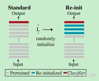
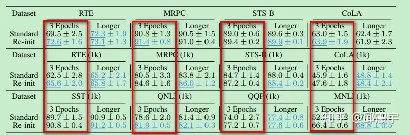
According to the experimental results, by reinitializing part of the weights, the model showed varying degrees of improvement in accuracy across four datasets. In addition, the authors conducted an experiment to verify how many layers’ weights should be reinitialized. The experimental results indicated that there is no significant rule; in fact, the number of layers to be initialized is related to the specific task and dataset, and needs to be determined through parameter tuning. However, one thing is certain: for classification tasks that require the pooler layer, reinitializing the pooler layer will certainly help the model’s training.
Further Verification
Similarly, I also verified the above idea in the CCKS named entity recognition competition. By fixing other parameters (including not using the bias-corrected Adam), I reinitialized the first 6 layers of BERT. The specific code implementation only requires filtering out the weights to be reinitialized from the assignment_map in the get_assignment_map_from_checkpoint method in modeling.py, as shown below:
def get_assignment_map_from_checkpoint(tvars, init_checkpoint):
    """Compute the union of the current variables and checkpoint variables."""
    assignment_map = {}
    initialized_variable_names = {}
    name_to_variable = collections.OrderedDict()
    for var in tvars:
        name = var.name
        m = re.match("^(.*):\d+$", name)
        if m is not None:
            name = m.group(1)
        name_to_variable[name] = var

    init_vars = tf.train.list_variables(init_checkpoint)

    assignment_map = collections.OrderedDict()
    filtered_layer_names = [......] // Here, just place the names of the weights to be reinitialized
    for x in init_vars:
        (name, var) = (x[0], x[1])
        if name not in name_to_variable:
            continue
        if name not in filtered_layer_names:
            assignment_map[name] = name_to_variable[name]
        initialized_variable_names[name] = 1
        initialized_variable_names[name + ":0"] = 1

    return (assignment_map, initialized_variable_names)
Through experiments, the above conclusions were verified. After reinitializing the weights of the top 6 layers of BERT, the model’s training efficiency significantly improved, with the convergence speed accelerating by 30-40%. However, the final model accuracy did not seem to change much, suggesting that the optimal number of layers for reinitialization still needs to be adjusted based on the validation set to achieve accuracy improvement.
Fine-tuning with Longer Steps
This optimization content seems to have no significant highlights. The author’s point is that increasing the number of training steps can enhance the fine-tuning effect. However, I generally use an early-stopping mechanism to control the number of training steps, so I won’t elaborate on this content further.
More Comparative Experiments
At the end of the paper, a set of comparative experiments was conducted, listing several classic methods for solving training oscillations, as follows:
1. Pre-trained Weight Decay: In traditional weight decay, the weight parameters are reduced by a regularization term  . In pre-trained weight decay, the pre-trained weights
  are introduced into the weight decay calculation during fine-tuning, making the final regularization term
  . This approach stabilizes model training.
2. Mixout: During fine-tuning, a probability p is set for each training iteration, allowing the model to randomly replace model parameters with pre-trained weight parameters according to this p. This method is primarily to alleviate catastrophic forgetting, ensuring the model does not forget the knowledge learned during pre-training during fine-tuning tasks.
3. Layerwise Learning Rate Decay: This method is one I often try, where different learning rates are used for different layers. Since the lower layers learn more general knowledge, they do not need to update parameters excessively during fine-tuning. Conversely, the upper layers, which are more inclined to learn task-related knowledge, require more updates.
4. Transferring via an Intermediate Task: This method involves fine-tuning on a larger transitional task before fine-tuning a small sample dataset task.
The author conducted comparative experiments between the above four methods and several optimization points in this paper, ultimately finding that compared to using only the bias-corrected Adam optimization algorithm, Pre-trained Weight Decay, Mixout, and Layerwise Learning Rate Decay did not show significant advantages. When combining bias correction and weight reinitialization, the effects of the above three methods were notably different. As for Transferring via an Intermediate Task, although it performed well, it requires additional labeled data, which is costly. I have also conducted some verification tests, using the MSRA Chinese NER dataset for fine-tuning, and then attempting to use its weight parameters for the CCKS NER task, but did not observe significant improvements. I personally believe that this transitional task needs to have a certain relevance to the target task’s domain; otherwise, domain transfer work is still needed.
Conclusion
This article mainly interprets the paper “Revisiting Few-sample BERT Fine-tuning”. By deeply studying the training instability issues encountered by BERT in fine-tuning small sample datasets, several optimization methods were proposed, including using the bias-corrected Adam optimization method and reinitializing partial weight parameters. The author conducted detailed experiments to verify these methods, and I also performed a simple secondary verification on a small sample task, ultimately proving the effectiveness of the aforementioned methods. Since these methods are very easy to implement with minimal changes to the original code, they are very suitable for application in practical projects.
This article is published on the public account platform with the author’s authorization, welcome to contribute, AI and NLP are both welcome.Original link, click “Read the original” to go directly:
https://zhuanlan.zhihu.com/p/148720604
Important! The PyTorch group for Yizhen Natural Language Processing has been established.
We have organized the official PyTorch Chinese tutorial.
Add the assistant to receive it, and you can also enter the official group!
Note: Please modify the remarks when adding to [School/Company + Name + Direction]
For example —— Harbin Institute of Technology + Zhang San + Dialogue System.
The account owner, please consciously avoid the micro-business. Thank you!

Recommended Reading:
NLP Learning (1) - Introduction to NER

NLP Learning (2) - Overview of NER

Softmax Function and Cross-Entropy