Join the professional CV group at Jishi, and interact with 10,000+ visual developers from top universities and companies like HKUST, Peking University, Tsinghua University, Chinese Academy of Sciences, CMU, Tencent, Baidu!

We also provide monthly live sharing sessions with experts, real project requirements matching, and a collection of valuable information for industry technical exchanges. Follow the Jishi Platform public account, reply with join group, and apply to join immediately~

Source | AI Algorithm Training Camp

What is the Attention Mechanism in Vision?

The basic idea of the attention mechanism in computer vision is to enable the system to learn to focus on important information while ignoring irrelevant information.

In recent years, most research combining deep learning with visual attention mechanisms has focused on using masks to form attention mechanisms. The principle of masks is to identify key features in image data through a new layer of weights, allowing the deep neural network to learn which areas of each new image need attention, thereby forming attention.

There are two types of attention mechanisms: soft attention and hard attention.

• The key point of soft attention is that it focuses more on regions or channels, and soft attention is deterministic. After learning, it can be generated directly through the network. The most critical aspect is that soft attention is differentiable, which is very important. Differentiable attention can calculate the gradient through the neural network and learn the attention weights through forward propagation and backward feedback.

• Hard attention differs from soft attention in that it focuses more on points, meaning that each point in the image can extend attention, and hard attention is a random prediction process that emphasizes dynamic changes. Of course, the key point is that hard attention is non-differentiable, and the training process is often completed through reinforcement learning.

In computer vision, many related works in various fields (such as classification, detection, segmentation, generative models, video processing, etc.) use Soft Attention. These works have also derived many different methods of using Soft Attention. The common part of these methods is that they utilize relevant features to learn weight distributions, and then apply the learned weights on the features to further extract relevant knowledge.

However, the way weights are applied varies slightly and can be summarized as follows:

• Weights can be applied to the original image;

• Weights can be applied on spatial scales, giving different spatial regions weights;

• Weights can be applied on channel scales, giving different channel features weights;

• Weights can be applied on historical features at different times, combining with recurrent structures to add weights, such as in machine translation or video-related tasks.

This article mainly focuses on the Self-attention mechanism and its application in visual applications—Non-local network module.

1. Self-Attention Mechanism in Visual Applications

1.1 Self-Attention Mechanism

Due to the local receptive field of the convolution kernel, it takes many layers to relate different parts of the entire image. Therefore, at the CVPR2018 conference, Hu J et al. proposed SENet, which statistically captures the global information of the image from the feature channel level. Here, we share another special form of Soft Attention—Self Attention.

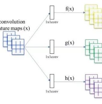
Self-Attention is an idea borrowed from NLP, thus retaining names like Query, Key, and Value. The following figure shows the basic structure of self-attention, where feature maps are obtained from basic deep convolutional networks such as ResNet, Xception, etc. These basic deep convolutional networks are referred to as the backbone, usually removing the last two downsampling layers of ResNet so that the obtained feature maps are 1/8 the size of the original input image.

The Self-attention structure is divided into three branches from top to bottom: query, key, and value. The computation is usually divided into three steps:

• The first step is to calculate the similarity between the query and each key to obtain weights. Common similarity functions include dot product, concatenation, and perceptron, etc.;

• The second step generally uses a softmax function to normalize these weights;

• The third step is to perform a weighted sum of the weights and the corresponding key values to obtain the final attention.

Next, we will explain the principle of self-attention through code.

class Self_Attn(nn.Module):
    """ Self attention Layer"""
    def __init__(self,in_dim,activation):
        super(Self_Attn,self).__init__()
        self.chanel_in = in_dim
        self.activation = activation

        self.query_conv = nn.Conv2d(in_channels = in_dim , out_channels = in_dim//8 , kernel_size= 1)
        self.key_conv = nn.Conv2d(in_channels = in_dim , out_channels = in_dim//8 , kernel_size= 1)
        self.value_conv = nn.Conv2d(in_channels = in_dim , out_channels = in_dim , kernel_size= 1)
        self.gamma = nn.Parameter(torch.zeros(1))

        self.softmax  = nn.Softmax(dim=-1)
    def forward(self,x):
        """
            inputs :
                x : input feature maps( B X C X W X H)
            returns :
                out : self attention value + input feature
                attention: B X N X N (N is Width*Height)
        """
        m_batchsize,C,width ,height = x.size()
        proj_query  = self.query_conv(x).view(m_batchsize,-1,width*height).permute(0,2,1) # B X CX(N)
        proj_key =  self.key_conv(x).view(m_batchsize,-1,width*height) # B X C x (*W*H)
        energy =  torch.bmm(proj_query,proj_key) # transpose check
        attention = self.softmax(energy) # BX (N) X (N)
        proj_value = self.value_conv(x).view(m_batchsize,-1,width*height) # B X C X N

        out = torch.bmm(proj_value,attention.permute(0,2,1) )
        out = out.view(m_batchsize,C,width,height)

        out = self.gamma*out + x
        return out,attention

Assuming the size of the feature maps is Batch_size×Channels×Width×Height

In the initialization function, three 1×1 convolutions are defined, namely query_conv, key_conv, and value_conv:

• In the query_conv convolution, the input is B×C×W×H, and the output is B×C/8×W×H;

• In the key_conv convolution, the input is B×C×W×H, and the output is B×C/8×W×H;

• In the value_conv convolution, the input is B×C×W×H, and the output is B×C×W×H.

In the forward function, the specific steps of self-attention are defined.

Step One:

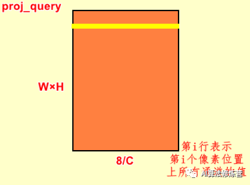
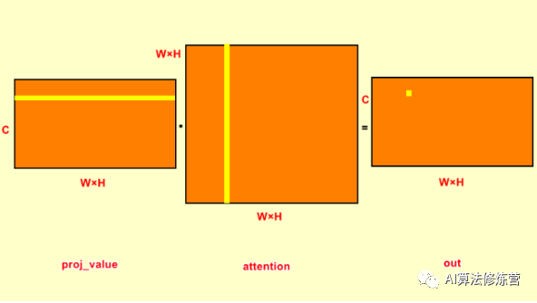
proj_query  = self.query_conv(x).view(m_batchsize,-1,width*height).permute(0,2,1)

proj_queryis essentially a convolution, but with a reshape operation added. First, the input feature map is convolved with query_conv, producing an output of B×C/8×W×H; the view function changes the output dimensions, pulling the W×H size flat to 1×(W×H); for a single feature map, the output is B×C/8×(W×H); the permute function then swaps the second and third dimensions, resulting in an output of B×(W×H)×C/8. The i-th row in proj_query represents the values of all channels at the i-th pixel position.

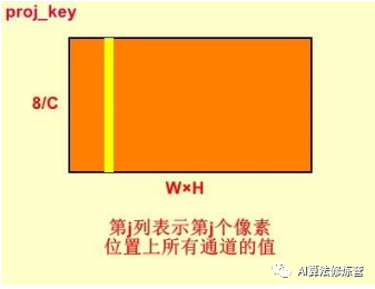
proj_key =  self.key_conv(x).view(m_batchsize,-1,width*height)

proj_key is similar to proj_query, but without the final inversion, resulting in an output of B×C/8×(W×H). The j-th row in proj_key represents the values of all channels at the j-th pixel position.

Step Two:

energy =  torch.bmm(proj_query,proj_key)

This step performs matrix multiplication on each pair of proj_query and proj_key in the batch_size, resulting in an output of B×(W×H)×(W×H). The element at position (i,j) in energy is obtained by dot multiplying the i-th row of proj_query with the j-th row of proj_key. The significance of this step is that the element at position (i,j) in energy indicates the influence of the j-th element in the input feature map on the i-th element, thereby achieving the dependency relationship between any two elements in the global context.

Step Three:

attention = self.softmax(energy)

This step applies softmax normalization to energy, which is normalization across rows. After normalization, the sum of each row equals 1, and for position (i,j), it can be understood as the weight of the j-th position on the i-th position, where the sum of all weights for the i-th position equals 1, thus obtaining the attention_map.

proj_value = self.value_conv(x).view(m_batchsize,-1,width*height)

proj_value is similar to proj_query and proj_key, except that the input is B×C×W×H, resulting in an output of B×C×(W×H). From the self-attention structure diagram, we can see that proj_value is multiplied by the attention_map, as shown in the following two lines of code.

out = torch.bmm(proj_value,attention.permute(0,2,1) )
out = out.view(m_batchsize,C,width,height)

Before performing the dot product between proj_value and attention_map, we first transpose attention. This is because the sum of each row in attention equals 1, representing the weight of the j-th position in the original feature map on the i-th position. After transposing, the sum of each column equals 1; the rows of proj_value are dot-multiplied with the columns of attention, applying weights to proj_value, resulting in an output of B×C×(W×H).

# Step Four:
out = self.gamma*out + x

This step performs weighting on the output after attention, where x is the original feature map, adding it to the original feature map. Gamma is learned, initially set to 0, resulting in the original feature map; as learning progresses, attention is weighted and added to the original feature map, resulting in the global dependency relationship between any two positions in the feature map.

1.2 Application of Self-Attention Mechanism: Non-local Neural Networks

Paper Link:https://arxiv.org/abs/1711.07971

Code Link:https://github.com/pprp/SimpleCVReproduction/tree/master/attention/Non-local/Non-Local_pytorch_0.4.1_to_1.1.0/lib

In the field of computer vision, an important paper on Attention research, Non-local Neural Networks, proposes a self-attention mechanism for non-local information statistics based on capturing the dependency relationships between long-range features.

The paper lists three issues that arise when convolutional networks statistically capture global information as follows:

1. Capturing long-range feature dependencies requires accumulating many layers of the network, leading to very low learning efficiency;

2. Since the network needs to accumulate many layers, careful design of modules and gradients is necessary;

3. When messages need to be passed back and forth between distant positions, it is difficult for convolutional or sequential local operations.

Therefore, the authors proposed a generalized, simple, and directly embeddable non-local operation operator based on the idea of non-local means filtering in image filtering, which can capture long-range dependencies in time (one-dimensional sequential signals), space (images), and spatiotemporal (video sequences). The benefits of this design are:

• Compared to continuously stacking convolutional and RNN operators, non-local operations can quickly capture long-range dependencies by directly computing the relationship between two positions (which can be temporal, spatial, or spatiotemporal), although it ignores their Euclidean distance. This computation method is essentially calculating the autocorrelation matrix, which is a generalized autocorrelation matrix;

• Non-local operations are highly efficient; to achieve the same effect, fewer stacked layers are needed;

• Non-local operations can ensure that the input scale and output scale remain unchanged, making it easy to embed into current network architectures.

Next, we will analyze how the authors handle long-distance information.

Non-local block

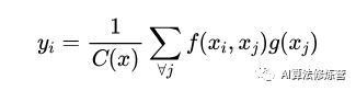
The general formula for Non-local is represented as:

• x is the input signal, generally a feature map used in CV
• i represents the output position, such as spatial, temporal, or spatiotemporal indices, and its response should be calculated by enumerating j
• f is a function that calculates the similarity between i and j
• g is a function that calculates the representation of the feature map at position j
• The final y is obtained after standardization by the response factor C(x)

It can be seen that, similar to Non-local mean calculation, i represents the response at the current position, while j represents the global response, obtained through weighting to get a non-local response value.

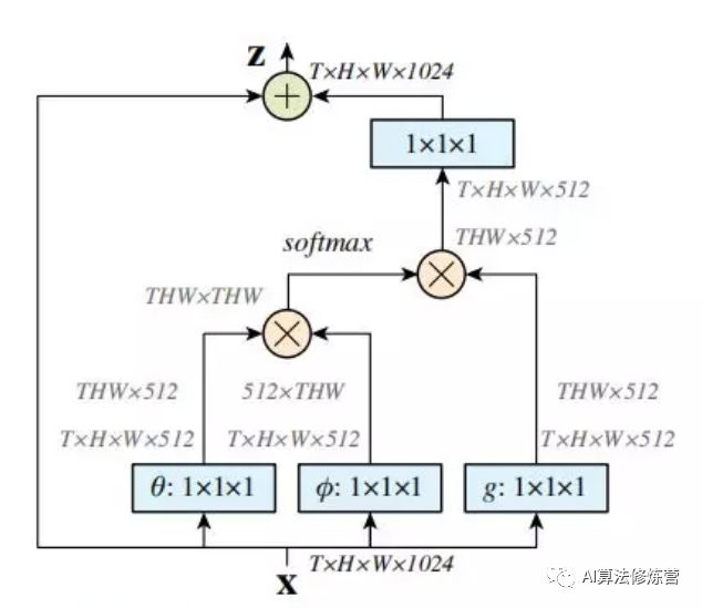
The paper discusses various implementation methods; here we briefly introduce the Matmul method, which is best implemented in DL frameworks (as shown in the Non-local block above):

1. First, perform linear mapping on the input feature map X (essentially a 1*1*1 convolution to compress the number of channels), obtaining θ, φ, and g features;

2. By reshaping, forcefully merging the dimensions of the above three features excluding the number of channels, then perform matrix dot product operation between θ and φ to obtain something similar to a covariance matrix (this process is important, calculating the autocorrelation of features, i.e., obtaining the relationship of each pixel in each frame to all other pixels in all frames);

3. Then perform the Softmax operation on the autocorrelation features to obtain weights ranging from 0 to 1, which are the Self-attention coefficients we need;

4. Finally, multiply the attention coefficients back to the feature matrix g, then expand the number of channels (1*1 convolution), and perform a residual operation with the original input feature map X to obtain the output of the non-local block.

Potential issues—high computational cost: Introducing non-local layers at the high-level semantic layer can also add pooling layers during implementation to further reduce computational costs.

import torch
from torch import nn
from torch.nn import functional as F


class _NonLocalBlockND(nn.Module):
    """
    Calling process
    NONLocalBlock2D(in_channels=32),
    super(NONLocalBlock2D, self).__init__(in_channels,
            inter_channels=inter_channels,
            dimension=2, sub_sample=sub_sample,
            bn_layer=bn_layer)
    """
    def __init__(self,
                 in_channels,
                 inter_channels=None,
                 dimension=3,
                 sub_sample=True,
                 bn_layer=True):
        super(_NonLocalBlockND, self).__init__()

        assert dimension in [1, 2, 3]

        self.dimension = dimension
        self.sub_sample = sub_sample

        self.in_channels = in_channels
        self.inter_channels = inter_channels

        if self.inter_channels is None:
            self.inter_channels = in_channels // 2
            # Compress to obtain the number of channels
            if self.inter_channels == 0:
                self.inter_channels = 1

        if dimension == 3:
            conv_nd = nn.Conv3d
            max_pool_layer = nn.MaxPool3d(kernel_size=(1, 2, 2))
            bn = nn.BatchNorm3d
        elif dimension == 2:
            conv_nd = nn.Conv2d
            max_pool_layer = nn.MaxPool2d(kernel_size=(2, 2))
            bn = nn.BatchNorm2d
        else:
            conv_nd = nn.Conv1d
            max_pool_layer = nn.MaxPool1d(kernel_size=(2))
            bn = nn.BatchNorm1d

        self.g = conv_nd(in_channels=self.in_channels,
                         out_channels=self.inter_channels,
                         kernel_size=1,
                         stride=1,
                         padding=0)

        if bn_layer:
            self.W = nn.Sequential(
                conv_nd(in_channels=self.inter_channels,
                        out_channels=self.in_channels,
                        kernel_size=1,
                        stride=1,
                        padding=0), bn(self.in_channels))
            nn.init.constant_(self.W[1].weight, 0)
            nn.init.constant_(self.W[1].bias, 0)
        else:
            self.W = conv_nd(in_channels=self.inter_channels,
                             out_channels=self.in_channels,
                             kernel_size=1,
                             stride=1,
                             padding=0)
            nn.init.constant_(self.W.weight, 0)
            nn.init.constant_(self.W.bias, 0)

        self.theta = conv_nd(in_channels=self.in_channels,
                             out_channels=self.inter_channels,
                             kernel_size=1,
                             stride=1,
                             padding=0)
        self.phi = conv_nd(in_channels=self.in_channels,
                           out_channels=self.inter_channels,
                           kernel_size=1,
                           stride=1,
                           padding=0)

        if sub_sample:
            self.g = nn.Sequential(self.g, max_pool_layer)
            self.phi = nn.Sequential(self.phi, max_pool_layer)

    def forward(self, x):
        '''
        :param x: (b, c,  h, w)
        :return:
        '''

        batch_size = x.size(0)

        g_x = self.g(x).view(batch_size, self.inter_channels, -1)#[bs, c, w*h]
        g_x = g_x.permute(0, 2, 1)

        theta_x = self.theta(x).view(batch_size, self.inter_channels, -1)
        theta_x = theta_x.permute(0, 2, 1)

        phi_x = self.phi(x).view(batch_size, self.inter_channels, -1)
        
        f = torch.matmul(theta_x, phi_x)

        print(f.shape)

        f_div_C = F.softmax(f, dim=-1)

        y = torch.matmul(f_div_C, g_x)
        y = y.permute(0, 2, 1).contiguous()
        y = y.view(batch_size, self.inter_channels, *x.size()[2:])
        W_y = self.W(y)
        z = W_y + x
        return z	

Non-local NN is inspired by the traditional method of Non-local means, and then applies this idea in neural networks, directly integrating global information rather than obtaining relatively global information merely by stacking multiple convolutional layers. This can provide richer semantic information for subsequent layers.

The paper also demonstrates the effectiveness of this module in video classification, object detection, instance segmentation, keypoint detection, etc., through ablation experiments. However, it does not provide changes in parameter amounts or computational speed. It can be inferred that the increase in parameter amounts is certain; for experiments with speed requirements, a trade-off between speed and accuracy may be necessary, and non-local blocks should not be added blindly. Another common operation in neural networks that also utilizes global information is the Linear layer; the fully connected layer integrates information from every point on the feature map, and Linear can be seen as a special non-local operation.

However, the Non-local Neural Networks module still has the following shortcomings:

  (1) It only involves the position attention module, without addressing the commonly used channel attention mechanisms

  (2) It can be seen that if the feature map is large, then multiplying two matrices of size (batch,hxw,512) is very memory and computation-intensive, meaning that when input feature maps are large, there are efficiency issues, although there are other ways to solve this, such as scaling, but this will lose information and is not the best solution.

Improvement Ideas

Recommended Reading:

• Application of Attention Mechanism in Classification Networks: SENet, SKNet, CBAM

• Stronger than CNN, the team led by Jia Jiaya from CUHK proposes two new types of self-attention networks | CVPR2020

• Attention Overview: Basic Principles, Variants, and Recent Research