Abstract: With the rapid development of communication technology today, the electromagnetic space environment has become increasingly complex, and the types of signals in the electromagnetic space have also diversified. Faced with various interferences in the electromagnetic space, accurately and effectively distinguishing the types of electromagnetic signals has become more challenging. To address this issue, a method for electromagnetic signal recognition based on a fusion model of Convolutional Neural Networks and Transformer networks is proposed. This method generates a network model structure oriented towards electromagnetic signals through the design of convolutional network structure and model parameters, and then integrates the Transformer network with the proposed Convolutional Neural Network to analyze the performance of electromagnetic signal recognition using the public dataset RadioML2016.10a. Experimental results show that the proposed novel network model has better recognition performance for electromagnetic signals compared to existing popular neural network models, making it more suitable for applications in electromagnetic signal recognition.
0 Introduction
The rapid development of communication technology has brought great convenience to people’s lives and is an important guarantee for meeting people’s material and cultural needs. However, with the exponential growth of communication data, limited spectrum resources have become increasingly tight, making effective allocation, management, and use of spectrum resources one of the important research topics in the field of communication. Therefore, communication signal recognition plays a crucial role in the current information and communication field and also plays an important role in both civilian and military domains. In the civilian sector, signal recognition technology is widely used in the monitoring and management of the electromagnetic spectrum; in the military sector, correctly identifying electromagnetic signals can provide electronic intelligence support for reconnaissance devices and has broad applications in electronic support systems, electronic intelligence systems, and radar threat warning systems.
Deep learning is a data-driven artificial intelligence method that can automatically mine data features and classify and recognize them. In the past decade, deep learning has achieved remarkable results in fields such as speech recognition and image retrieval. Recent studies have shown that Convolutional Neural Networks (CNN) have significantly improved in many areas, including target detection, image classification and segmentation, and radio signal classification recognition.
In 2016, to achieve automatic modulation recognition of radio signals under low signal-to-noise ratios, O’Shea et al. used a software-defined radio platform GUN Radio to generate a dataset of radio signals, with a dynamic range of signal-to-noise ratios from -20 to 18 dB, and input all time-domain data under all signal-to-noise ratios into the CNN network model for modulation recognition. Experimental results showed that the recognition performance of the CNN trained on baseband I and Q data was higher than that of the modulation recognition algorithm based on cyclic matrices. Mendis et al. used the Spectral Correlation Function (SCF) to convert baseband signals into image signals and conducted modulation recognition experiments using deep learning network models. Experimental results indicated that this algorithm outperformed recognition algorithms based on deep learning network models of baseband signals. In 2018, O’Shea generated a larger range of modulation signal datasets based on the RadioML2016.10a dataset, increasing the types of signals to 24; O’Shea proposed a modulation recognition algorithm using Residual Networks (ResNet) and determined the network structure and parameters through simulation experiments. To address the issue of wideband spectrum signals being difficult to identify due to wide frequency bands and limited receiver sampling steps in the field of spectrum monitoring, Zhou Yuhang et al. proposed a method combining frequency domain stacking preprocessing and target detection for spectrum signal recognition. This method utilizes frequency domain stacking to highlight weak signals in the spectrum and sends the processed spectrum images into an improved target detection network for signal type recognition. Some researchers have even transformed signal problems into image problems. Experiments by Peng et al. showed that models based on three-channel constellation diagrams and CNN outperformed traditional modulation signal recognition algorithms and constellation-based modulation signal recognition methods. Zhou Xin et al. proposed a method using image deep learning to process radio signals, enhancing the automation level of radio signal discrimination and judgment in complex electromagnetic spaces. However, most of the above methods focus on processing and altering signal designs rather than designing network structures specifically for electromagnetic signals.
Transformer is a network structure based on a self-attention mechanism, first proposed by Google in 2017. It has since shown outstanding results in natural language processing, and its application has gradually become a pillar in deep learning after demonstrating remarkable performance in computer vision.
In the field of image and video, standalone Transformer architectures are primarily used in benchmark testing, with more variants and combinations continuously emerging. Zamir et al. proposed an efficient Transformer model that captures long-distance pixel interactions through several key designs in the constructed multi-head attention and feedforward network blocks while remaining applicable to large images, demonstrating outstanding performance in image restoration. In the speech domain, Gulati et al. proposed a convolution-enhanced transformer model, Conformer, which outperformed standalone Transformers and CNN-based network models, achieving state-of-the-art accuracy.
Most applications of Transformers have been in natural language processing, computer vision, and speech recognition, with minimal applications in electromagnetic signal recognition, and there has been little progress in proposing network models specifically for electromagnetic signals. Therefore, this paper combines the advantages of CNN’s local perception and Transformer’s global perception to propose a CNN-Transformer-based network model for electromagnetic signal recognition and analyze the characteristics of this model in signal recognition performance.
1 Network Model Structure Parameter Optimization
The network structure proposed in this paper consists of two main parts: the CNN network model and the Transformer network model. The entire CNN-Transformer network model clearly distinguishes categories of electromagnetic signals through capturing local information of feature data and perceiving global features.
1.1 CNN Model Structure Parameters
CNN is essentially composed of variants of Multi-layer Perceptrons (MLP), and its success lies in the adoption of weight sharing and local connections, which not only reduces the number of weights, making the network model easier to optimize, but also lowers the model’s complexity, thereby reducing the potential risk of overfitting. The core module of the low hidden layer structure of CNN mainly consists of convolutional layers and pooling layers, while the core module of the high hidden layer is replaced by fully connected layers instead of traditional MLP hidden layers and classifiers.
1.1.1 Convolutional Layer
The neural units in CNN are interconnected through convolution operations, and the network model internally performs feature extraction on the input data through convolution operations sequentially. Let’s assume each convolutional layer has n convolution kernels; different sizes of convolution kernels extract local features from the input data differently, ultimately resulting in n sets of output data, referred to as feature maps. If the number of convolution kernels in the convolutional layer increases, the features extracted from the input data also increase, thereby enhancing its representation capability for features.
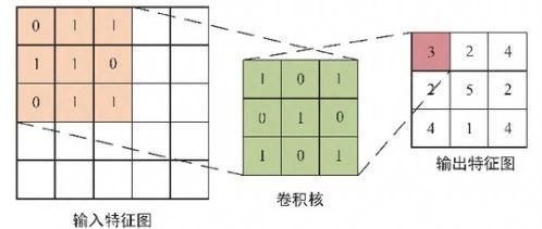
As shown in Figure 1, if the size of the convolution kernel is 3, the convolutional layer completes local feature extraction through convolution operations and then moves on the feature map according to a certain stride to perform convolution operations, finally completing all feature extraction tasks. Assuming the dimension of the feature map is MxN, the size of the convolution kernel is IxJ, the expression for the convolution operation is: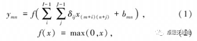
Where y is the value corresponding to the position (m,n) of the output feature map, x(m+i)(n+j) is the value corresponding to the position (m+i,n+j) of the input feature map, δ„ is the weight at the position (i,j) of the convolution kernel, bm is the corresponding bias, and f(x) is the nonlinear activation function Rectified Linear Unit (ReLU).
1.1.2 Pooling Layer
Compared to traditional neural networks, the setup of convolutional layers can effectively extract feature information from feature maps and reduce network parameters. However, the results after convolution operations still have high dimensions. To address this issue, the concept of the pooling layer has been introduced, which is generally connected after the convolutional layer. Its function is to perform sampling processing on the feature map processed by the convolutional layer, i.e., extracting values that can represent the features of that area within different sub-regions, achieving a reduction in the size and dimensionality of the feature map while retaining the basic information of the features, thus lowering network complexity and preventing overfitting. Additionally, for signal features, the relative position of feature details is more important, and the pooling layer enhances the translation invariance of neural network recognition.
The pooling layer is generally divided into two types: max pooling and average pooling. This paper chooses max pooling, where the neighborhood area of the max pooling layer is rectangular, taking the maximum value of that neighborhood as the output of the pooling layer. The schematic diagram of max pooling is shown in Figure 2. The size of the pooling layer can be adjusted according to actual needs.
1.1.3 Batch Normalization Layer
Batch Normalization (BN) is a widely used training technique in deep learning network models. On one hand, it can improve the convergence speed of the model; on the other hand, it simplifies the initialization requirements, allowing for larger learning rate parameters.
1.2 Transformer Structure
Transformer is essentially an Encoder-Decoder architecture. Therefore, the middle part of the Transformer can be divided into two parts: the encoding component and the decoding component.
As shown in Figure 3, the left part is the encoding component, mainly composed of multi-head self-attention mechanisms and feedforward neural networks. The right part is the decoding component, mainly consisting of masked self-attention mechanisms, multi-head self-attention mechanisms, and feedforward neural networks.
2 CNN-Transformer Network Fusion Model Electromagnetic Signal Recognition Process Design
2.1 Model Framework
The overall framework of the CNN-Transformer network fusion model is shown in Figure 4, mainly including data preparation module, parameter optimization module, and prediction training module. This paper optimizes the design of the network model by adjusting the number of convolutional layers, the size of convolution kernels, the position of pooling layers, and the presence or absence of batch normalization layers, obtaining a suitable CNN model and integrating it with the Transformer network model to form a new network model for electromagnetic signal recognition experiments. The process for electromagnetic signal recognition is as follows:
Step 1: Preprocess the dataset and label it;
Step 2: Optimize the design direction by selecting pooling layer positions, convolution kernel sizes, and the number of convolutional layers, and whether to include batch normalization layers;
Step 3: Train the dataset in conjunction with the Transformer network model;
Step 4: Obtain the results of electromagnetic signal recognition through the test set.
2.2 Data Preprocessing
This paper uses the public dataset RadioML2016.10a, which was collected through GNU devices in real scenarios and contains 11 types of signals with various channel impairments. Specific data parameters are shown in Table 1.
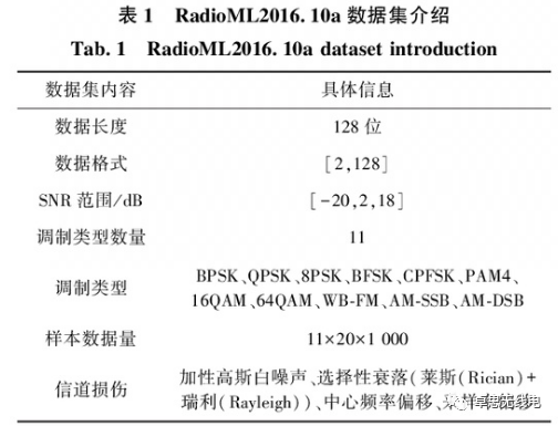
To enable the model to effectively process the dataset, the data is divided into three parts: training set, validation set, and test set, with a ratio of 8:1:1. At the same time, the one-hot encoding algorithm labels each data point with the corresponding signal for recognition. Finally, the data format is rearranged to [128,2] for easier transmission into the network model. Since the data itself has been normalized, this paper does not perform normalization on the data.
2.3 Network Model Design
First, a shallow CNN2 is used as the design basis, with its structure shown in Table 2.
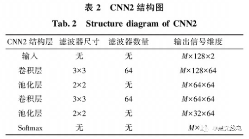
By studying the positions of pooling layers, pooling layers are set after 1 to 4 convolutional layers to ensure that feature information can be fully extracted, thus determining the optimal position for the pooling layer. Similarly, convolution kernels are set to sizes of 1×1, 2×2, 3×3, and 4×4 to determine which size is more suitable for electromagnetic signals. Convolution blocks are composed of several convolutional layers and one pooling layer, and the number of convolution blocks is set to 2 to 5 to determine which configuration is more suitable for electromagnetic signals. By setting the presence or absence of a batch normalization layer, the impact of batch normalization on electromagnetic signal recognition can be determined. The designed model is then compared with existing classical centralized neural network models to demonstrate its recognition performance.
Finally, the CNN network and Transformer model are sequentially fused to recognize electromagnetic signals and obtain research results.
3 Experiments and Performance Analysis
3.1 Environment Configuration
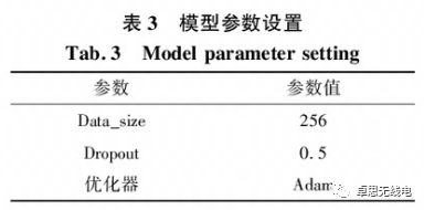
The parameters of the CNN model are shown in Table 3. To prevent model overfitting, a Dropout layer is added after each fully connected layer, with a dropout rate set to 0.5. The Adam optimizer is selected to automatically apply a custom learning rate to the model parameters, improving training convergence performance.
The computer configuration used for the experiment is: Intel(R) Core(TM) i7-10750H CPU @ 2.60 GHz processor, 16 GByte memory, Windows (64-bit) operating system, software development environment Python 3.8 and PyTorch.
3.2 NN Model Performance Analysis
The CNN model design is based on CNN2, and the impacts of different parameters and structural designs have been analyzed.
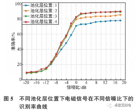
3.2.1 Pooling Layer Position
Referring to the CNN2 model, experiments on the design of pooling layers at different positions were conducted, as shown in Figure 5. From the figure, it can be seen that after 2 dB, all models’ recognition effects stabilize, and as the number of convolutional layers increases, the recognition rate also continues to rise. After reaching 3 convolution layers, further increasing the number of convolution layers does not enhance the recognition effect significantly, and the recognition effect is not much different from that at 3 layers, indicating that 3 convolution layers plus one pooling layer can adequately extract feature information from the signals.
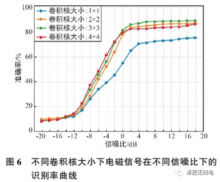
3.2.2 Size of Convolution Kernels
Convolution operations are essential for extracting feature information, and the size of convolution kernels is particularly important for feature extraction. As shown in Figure 6, it can be seen that when the signal-to-noise ratio reaches 4 dB, the recognition rate stabilizes; the effect is worst when the convolution kernel size is 1×1, while the best recognition effect is achieved with a kernel size of 3×3. However, when the kernel size is 4×4, the recognition effect deteriorates, indicating that when the convolution kernel is 3×3, the convolution operation can maximize the extraction of feature information from the signals; if the kernel is too large, it may extract insufficient local information, while if it is too small, it may fail to capture the correlation features between signals, resulting in poor recognition performance.
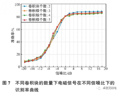
3.2.3 Size of Convolution Blocks
Without overfitting, deeper networks can better extract information for classification and recognition. As shown in Figure 7, when the signal-to-noise ratio reaches 2 dB, the recognition rate curve gradually stabilizes; when the number of convolution blocks is set to 2, the signal recognition effect is the best. However, as the number of convolution blocks increases, the signal recognition effect decreases; moreover, the recognition effects are quite similar, indicating that 2 convolution blocks are the most suitable. When the number of convolution blocks increases, excessive convolution operations may extract more pronounced feature information, thereby neglecting some subtle features, resulting in poorer recognition performance compared to before.
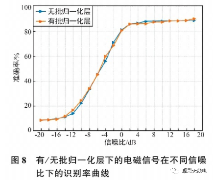
3.2.4 Batch Normalization Layer
The recognition rate curves of electromagnetic signals under different signal-to-noise ratios with and without batch normalization layers are shown in Figure 8. It can be seen that after the signal recognition rate stabilizes, the recognition effects of models with and without batch normalization layers are not much different, indicating that the presence or absence of a batch normalization layer does not affect signal recognition. The reason may be that the dataset has already undergone batch normalization processing, so adding a batch normalization layer has little impact on the experimental results.
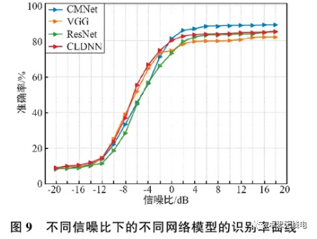
3.2.5 Model Performance Comparison Analysis
After designing the model parameters and structure, with pooling layers composed after 3 convolution layers, a convolution kernel size of 3×3, and 2 convolution blocks without batch normalization layers, a comparison with VGG, ResNet, and CLDNN is shown in Figure 9. It can be seen that when the signal-to-noise ratio is 2 dB, the recognition rate stabilizes, and the recognition effect of the newly designed model is better than that of the other three network models, achieving a maximum recognition rate of 88.49%, which is 3.9% higher than the best-performing CLDNN among the other three networks, indicating that this network model has excellent performance for electromagnetic signal recognition.
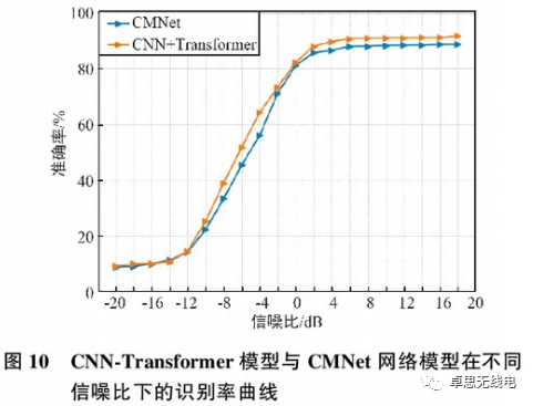
3.3 CNN-Transformer Model Performance Analysis
By integrating the completed CNN model with the Transformer model for signal recognition, as shown in Figure 10, when the signal-to-noise ratio is 2 dB, the signal recognition rate components begin to stabilize. The recognition effect of the fusion model is better than that of the designed convolutional neural network model, achieving a recognition rate of 91.2%, which is about 3% higher than that of the designed convolutional neural network model. This indicates that the addition of the Transformer structure successfully leverages the global perception capability of the Transformer to improve the model’s recognition performance, and the variety of Transformer model variants provides room for further optimization and improvement in future experiments.
4 Conclusion
Due to the lack of specific network structures and parameters proposed for deep learning models aimed at electromagnetic signals, the proposed model structure has developmental potential for electromagnetic signal recognition performance. To address this issue, this paper proposes an electromagnetic signal recognition method based on a fusion model of CNN and Transformer networks. This method redesigns the structure and parameters of CNN while utilizing the local feature capturing ability of CNN and the global information perception of the Transformer structure, resulting in a novel neural network model with good performance for electromagnetic signal recognition. This model has significant advantages in recognition performance compared to some classical network models. Additionally, due to the diversity of Transformer structure variants and the combination with CNN models, there is promising research potential for network structures aimed at electromagnetic signal recognition in the future.
Disclaimer: This article is an online excerpt or reprint, and the copyright belongs to the original author. The content reflects the personal views of the original author and does not represent the views of this public account or its responsibility for the authenticity of the content. If there are any copyright issues regarding the works, please contact us, and we will delete the content promptly!