MTF-CNN-Attention Fault Recognition Program

Applicable Platform: Matlab 2023 and above

This program references the ChineseEIJournal“Power Grid Technology” online publication, literature: “Classification Method of Power Quality Disturbances Based on Markov Transition Field and Multi-Head Attention Mechanism“. The program is well-commented and full of valuable content. Below is a brief introduction to the article and the program!

MTF-CNN-Attention Fault Recognition Program

Innovations in the Literature:The innovation of this literature lies in the combination of Markov Transition Field (MTF) and Convolutional Neural Network (CNN), incorporating a multi-head attention mechanism to achieve fault classification.MTF converts one-dimensional signals into two-dimensional feature maps, whileCNN can adaptively extract and classify features from these maps. The integration of the multi-head attention mechanism effectively captures the contribution of the extracted features, enabling accurate fault classification.

Fault Recognition Process:

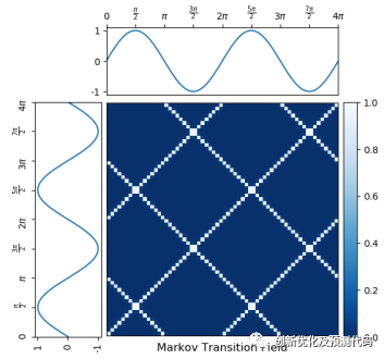
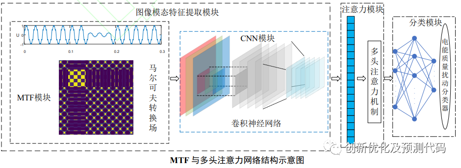Principle: Markov Transition Field (Markov transition field, MTF) is a method for transforming time-series data into spatial image data. This method extends the Markov state transition matrix by sequentially expressing the state transition matrix, fully preserving the dynamic information of the discretized time domain, and ultimately generating a two-dimensional image using fuzzy kernel aggregation. For example, the schematic diagram ofMTF is shown below.

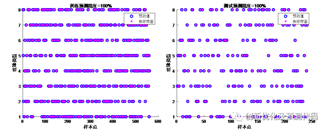
The MTF-CNN-Attention method for fault recognition has several innovative aspects:

Innovation in Data Representation: Typically, one-dimensional sequences (such as time series data) are used directly for modeling and analysis. Transforming these sequences into Markov field images is, in fact, a new method of data representation. This transformation may reveal new patterns and structural features in the sequence data that may not be as apparent or difficult to detect in their original one-dimensional form, capturing complex patterns and anomalies more effectively than traditional time-series analysis methods.

Image Processing Techniques: By converting sequence data into images, established image processing techniques and image recognition algorithms can be leveraged to analyze the data. This includes using various image recognition methods, such as Convolutional Neural Networks (CNN), which have proven to be very effective in image analysis but are not commonly used in traditional sequence data analysis.

Capturing Temporal Dependencies: Markov fields are a mathematical model used to represent the dependencies between random variables. When transforming sequence data into Markov field images, temporal dependencies and dynamic changes in the time series can be captured in image form, providing a new perspective for understanding and identifying fault patterns in time series.

Multi-Head Attention Mechanism:The integration of the multi-head attention mechanism effectively captures the contribution of the extracted features, enhancing the accuracy of fault recognition.

Program Application: Markov Transition Field (MTF) generates two-dimensional images from one-dimensional time series, then uses CNN to extract high-dimensional features from the images, and applies the Multihead Self-Attention mechanism to enhance the features, thereby improving the accuracy of fault recognition.

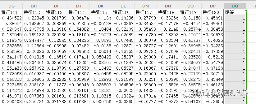
Input Data Format:(One sample per line, the last column indicates the fault category label)

Generating MTF Images from the Above Data:

Recognition Results: (Confusion Matrix for Training and Test Sets)

Scatter Plot for Training and Test Sets:

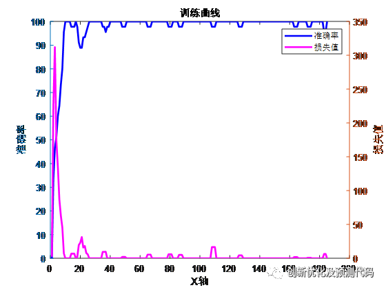
Training Curve: Accuracy and Loss Variation Chart

Markov Field Generation Partial Program:

% Load data
data = xlsread('FeatureDataWithLabels.xlsx');
% Get the number of samples and the length of each sample
[numSamples, sampleLength] = size(data);
% Loop through each sample data
for sampleIdx = 1:numSamples    %% Generate data    % Get current sample data from data    featureData = data(sampleIdx, 1:end - 1);
    X = featureData;    m = length(X);         % Normalize data to [0, 1]    X_normalized = (X - min(X)) / (max(X) - min(X));         %% Construct transition matrix W    numDataPoints = length(X);         % Divide into Q quantile bins (by count), from small to large: 1, 2, 3, 4    Q = 4;         % Map each element to quantile bins 1, 2, 3, 4    X_Q = ones(1, numDataPoints);    threshold = 0;         % Initialize threshold    thresholds = ones(1, Q + 1);    for i = 2 : Q + 1                % Loop to calculate the number of data points less than the current threshold, exit loop when threshold is reached        while sum(X_normalized < threshold) < numDataPoints * (i - 1) / Q            threshold = threshold + 0.0001;        end                % Record the threshold for each quantile bin        thresholds(i) = threshold;                % Transform original data vector into corresponding quantile order vector        X_Q(find(X_normalized < thresholds(i) & X_normalized > thresholds(i - 1))) = i - 1;    end         %% Calculate Markov matrix    % Initialize state transition counts    sum_11 = 0; sum_12 = 0; sum_13 = 0; sum_14 = 0;    sum_21 = 0; sum_22 = 0; sum_23 = 0; sum_24 = 0;    sum_31 = 0; sum_32 = 0; sum_33 = 0; sum_34 = 0;    sum_41 = 0; sum_42 = 0; sum_43 = 0; sum_44 = 0;

Some images are sourced from the internet; please contact for removal if infringement occurs!

Complete code:https://mbd.pub/o/bread/ZZial5lx

Welcome to interested friends to click “Read the Original“ or the link above to obtain the complete code~, follow the editor for more quality learning materials and article program codes~

Leave a Comment Cancel reply