Click the "Beginner's Visual Learning" above, select "Star" or "Top"
Heavy content delivered to you first
Researchers proposed the concept of CNN (Convolutional Neural Networks) while studying image processing algorithms. Traditional fully connected networks are a black box - they take all inputs and pass each value through a dense network, then to a hot output. This seems to work for a small amount of input.
When we process an image of 1024x768 pixels, we input 3x1024x768 = 2359296 numbers (the RGB values for each pixel). A dense multilayer neural network with an input vector of 2359296 numbers has at least 2359296 weights for each neuron in the first layer - each neuron in the first layer has 2MB of weights. This was nearly impossible for processors and RAM in the 1990s and 2000s.
This led researchers to wonder if there was a better way to accomplish this task. The first and most important task in any image processing (recognition) is usually edge and texture detection. Next comes the identification and processing of real objects. It is clear that detecting textures and edges does not actually depend on the entire image. One needs to look at the pixels surrounding a given pixel to identify edges or textures.
Moreover, the algorithm used to identify edges or textures should be the same throughout the image. We cannot use different algorithms for the center of the image or any corner or side. The concept of edge or texture detection must be the same. We do not need to learn a new set of parameters for each pixel in the image.
This understanding led to the development of Convolutional Neural Networks. The first layer of the network consists of neurons that scan small patches of the image - processing a few pixels at a time. Typically, these are squares of 9, 16, or 25 pixels.
CNN effectively reduces the computational load. Small "filters/kernels" slide along the image, processing a small patch at a time. The processing required for the entire image is very similar, making it very efficient.
Although it was introduced for image processing, CNNs have been applied in many other fields over the years.
An Example
Now that we understand the basic concept of CNN, let's look at how it works with numbers. As we have seen, edge detection is a primary task for any image processing problem. Let’s see how CNNs are used to solve the edge detection problem.
On the left is the bitmap of a 16x16 monochrome image. Each value in the matrix represents the brightness of the corresponding pixel. We can see that this is a simple gray image with a square in the middle. When we try to convolve it with a 2x2 filter (middle image), we get a 14x14 matrix (right image).
The filter we selected can highlight the edges in the image. We can see in the matrix on the right that the values corresponding to the edges in the original image are high (positive or negative). This is a simple edge detection filter. Researchers have identified many different filters that can recognize and highlight various aspects of an image. In typical Convolutional Neural Network (CNN) model development, we let the network learn and discover these filters itself.
Important Concepts
Here are some important concepts we should understand before further using CNNs.
Padding
An obvious problem with convolution filters is that each step reduces the size of the matrix, thereby reducing the "information" - shrinking the output. Essentially, if the original matrix is N×N and the filter is F×F, the resulting matrix will be (N-F + 1)×(N-F + 1). This is because there are fewer pixels on the edges than in the middle of the image.
If we pad the image with (F - 1)/2 pixels on all edges, we can retain the size of N×N.
Thus, we have two types of convolution: Valid Convolution and Same Convolution. Valid essentially means no padding. Therefore, each convolution will lead to a reduction in size. Same Convolution uses padding to keep the size of the matrix.
In computer vision, F is usually odd. Odd F helps maintain the symmetry of the image and allows for a central pixel, which aids in applying uniform bias in various algorithms. Thus, 3x3, 5x5, and 7x7 filters are common. We also have 1x1 filters.
Strides
The convolutions we discussed above are continuous as they scan pixels continuously. We can also use strides - by skipping s pixels while moving the convolution filter over the image.
So, if we have an nxn image and an fx f filter and we convolve with stride s and padding p, the output size would be: ((n + 2p - f)/s + 1) x ((n + 2p - f)/s + 1)
Convolution vs. Cross-Correlation
Cross-correlation is essentially the convolution of a matrix flipped along the bottom diagonal. The flipping adds correlation to the operation. But in image processing, we do not flip it.
Convolution on RGB Images
Now we have an nxnx3 image, and we convolve with an fxfx3 filter. Thus, we have height, width, and number of channels in any image and its filter. At any time, the number of channels in the image must match the number of channels in the filter. The output of this convolution has width and height (n-f + 1) and 1 channel.
Multiple Filters
A 3-channel image convolved with a 3-channel filter results in a single-channel output. But we are not limited to one filter. We can have multiple filters - each filter produces a new output layer. Therefore, the number of channels in the input should match the number of channels in each filter. The number of filters and the number of output channels are the same.
Thus, we start with an image with 3 channels and end up with multiple channels in the output. Each of these output channels represents a certain aspect of the image captured by the corresponding filter. Therefore, it is also referred to as features rather than channels. In a real deep network, we also add a bias and a non-linear activation function like RelU.
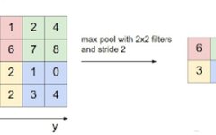
Pooling Layers
Pooling essentially combines values into one value. We can have average pooling, max pooling, min pooling, etc. Thus, using fx f pooling on nxn input will generate (n/f)x(n/f) output. It has no parameters to learn.
Max Pooling
CNN Architecture
Typical small to medium CNN models follow some basic principles.
Typical CNN Architecture
Alternating convolution and pooling layers
Gradually reducing frame size and increasing the number of frames,
Towards the end, flatten and fully connected layers
Activating RelU for all hidden layers, then softmax for the final layer
As we move towards large and super-large networks, things become increasingly complex. Researchers provide us with more specific architectures that can be used here (e.g., ImageNet, GoogleNet, and VGGNet).
Python Implementation
Typically when implementing a CNN model, we first perform data analysis and cleaning, then select the network model we can start with. We provide the architecture based on the number of networks and layer sizes and their connectivity layout - then we allow the network to learn the rest itself. Then we can adjust hyperparameters to generate a model sufficient to meet our purposes.
Let’s look at a simple example of how a convolutional network works.
Importing Modules
First, we import the required Python libraries.
import numpy as np
import tensorflow as tf
from tensorflow import keras
from keras.layers import Dense, Conv2D, Flatten, MaxPooling2D
from keras.models import Sequential
Getting Data
The next step is to get the data. We use the machine learning dataset built into the Keras module - the MNIST dataset. In real life, this requires more processing.
We load the training and testing data. We reshape the data to fit better into the convolutional network. Basically, we reshape it into a 4D array of size 60000 (number of records) by 28x28x1 (each image size is 28x28). This makes it easier to build Convolutional layers in Keras.
If we wanted a dense neural network, we would reshape the data into 60000x784 - a 1D record for each training image. But CNNs are different. Remember, the concept of convolution is 2D - so there is no need to flatten it into a 1D array.
We also change the labels to one-hot arrays for classification instead of numerical categories. Finally, we normalize the image data to reduce the likelihood of gradient vanishing.
(train_images, train_labels), (test_images, test_labels) = tf.keras.datasets.mnist.load_data()
train_images = train_images.reshape(60000,28,28,1)
test_images = test_images.reshape(10000,28,28,1)
test_labels = tf.keras.utils.to_categorical(test_labels)
train_labels = tf.keras.utils.to_categorical(train_labels)
train_images = train_images / 255.0
test_images = test_images / 255.0
Building the Model
The Keras library provides us with a ready-to-use API to build the model we want. We first create an instance of the Sequential model. Then we add layers to the model. The first layer is a convolutional layer that processes 28x28 input images. We define the kernel size as 3 and create 32 such kernels - creating 32 frames of output - size 26x26 (28-3 + 1 = 26)
Next is a 2x2 max pooling layer. This will reduce the size from 26x26 to 13x13. We used max pooling because we know the nature of the problem is edge-based - we know that edges show high values in convolution.
Next is another convolution layer with a kernel size of 3x3, generating 24 output frames. Each frame is of size 22x22. Next is the convolution layer. Finally, we flatten this data and input it into a dense layer, which has outputs corresponding to the 10 desired values.
model = Sequential()
model.add(Conv2D(32, kernel_size=3, activation='relu', input_shape=(28,28,1)))
model.add(MaxPooling2D(pool_size=(3, 3)))
model.add(Conv2D(24, kernel_size=3, activation='relu'))
model.add(MaxPooling2D(pool_size=(2, 2)))
model.add(Flatten())
model.add(Dense(10, activation='softmax'))
model.compile(optimizer='adam', loss='categorical_crossentropy', metrics=['accuracy'])
Training the Model
Finally, we train the machine learning model with the data we have. Five epochs are enough to get a fairly accurate model.
model.fit(train_images, train_labels, validation_data=(test_images, test_labels), epochs=5)
Download 1: OpenCV-Contrib Extension Module Chinese Tutorial
Reply "Extension Module Chinese Tutorial" in the "Beginner's Visual Learning" public account backend to download the first Chinese version of the OpenCV extension module tutorial, covering more than twenty chapters on extension module installation, SFM algorithms, stereo vision, object tracking, biological vision, super-resolution processing, etc.
Download 2: Python Visual Practical Projects 52 Lectures
Reply "Python Visual Practical Projects" in the "Beginner's Visual Learning" public account backend to download 31 visual practical projects, including image segmentation, mask detection, lane line detection, vehicle counting, eyeliner addition, license plate recognition, character recognition, emotion detection, text content extraction, facial recognition, etc., to help quickly learn computer vision.
Download 3: OpenCV Practical Projects 20 Lectures
Reply "OpenCV Practical Projects 20 Lectures" in the "Beginner's Visual Learning" public account backend to download 20 practical projects based on OpenCV to advance OpenCV learning.
Group Chat
Welcome to join the public account reader group to communicate with peers. There are currently WeChat groups for SLAM, 3D vision, sensors, autonomous driving, computational photography, detection, segmentation, recognition, medical imaging, GAN, algorithm competitions, etc. (will gradually subdivide in the future). Please scan the WeChat number below to join the group, with the remark: "Nickname + School/Company + Research Direction", e.g., "Zhang San + Shanghai Jiao Tong University + Visual SLAM". Please follow the format for remarks; otherwise, you will not be approved. After successful addition, you will be invited to relevant WeChat groups based on your research direction. Please do not send advertisements in the group; otherwise, you will be removed from the group. Thank you for your understanding~