Multi-Step Time Series Forecasting with LSTM

Long Short-Term Memory (LSTM) networks are a type of recurrent neural network capable of learning and predicting long sequences. In addition to learning long sequences, LSTMs can also learn to make multi-step predictions, which is very useful for time series forecasting. One challenge with LSTMs is that they can be difficult to configure and require a lot of preparation work to get the data in a format suitable for learning.

In this tutorial, you will learn how to develop an LSTM for multi-step time series forecasting using Keras in Python.

By the end of this tutorial, you will know:

• How to prepare data for multi-step time series forecasting.

• How to build an LSTM model for multi-step time series forecasting.

• How to evaluate a multi-step time series forecast.

Tutorial Overview

This tutorial is divided into four parts. They are:

• Shampoo Sales Dataset

• Data Preparation and Model Evaluation

• Persistence Model

• Multi-Step LSTM

Environment

This tutorial assumes that you have a Python SciPy environment installed. You can use either python2 or python3 for this example.

This tutorial also assumes that you have Keras v2.0 or higher installed, along with either the TensorFlow or Theano backend.

This tutorial further assumes that you have scikit-learn, pandas, NumPy, and Matplotlib installed.

Shampoo Sales Dataset

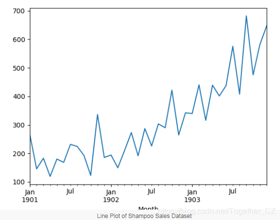
This dataset describes the monthly sales of shampoo over a period of three years. The units are sales counts, with 36 observations. The original dataset is credited to Makridakis, Wheelwright, and Hyndman (1998). You can download it here and learn more about the dataset. The example below loads and creates a plot of the loaded dataset.

Next, we will explore the model configuration and testing tools used in the experiment.

Data Preparation and Model Evaluation

This section describes the data preparation and model evaluation used in this tutorial.

Data Splitting

We will split the shampoo sales dataset into two parts: a training set and a test set. The training dataset will use the data from the first two years, while the test set will use the data from the last year. The model will be developed using the training dataset, and predictions will be made on the test dataset. The observations for the past 12 months are as follows:

"3-01",339.7
"3-02",440.4
"3-03",315.9
"3-04",439.3
"3-05",401.3
"3-06",437.4
"3-07",575.5
"3-08",407.6
"3-09",682.0
"3-10",475.3
"3-11",581.3
"3-12",646.9

Multi-Step Forecasting

We will design a multi-step forecast. For a given month in the last 12 months of the dataset, we need to make forecasts for the next three months. This is known as using historical observations (t-1, t-2, …, t-n) to forecast t, t+1, and t+2. Specifically, starting from December of the second year, we must forecast January, February, and March. From January, we must forecast February, March, and April. This continues until the forecasts for October, November, and December are made from September of the third year. In total, 10 forecasts of three months each are needed, as follows:

Dec, Jan, Feb, Mar
Jan, Feb, Mar, Apr
Feb, Mar, Apr, May
Mar, Apr, May, Jun
Apr,  May, Jun, Jul
May, Jun, Jul, Aug
Jun, Jul, Aug, Sep
Jul, Aug, Sep, Oct
Aug, Sep, Oct, Nov
Sep, Oct, Nov, Dec

Model Evaluation

Rolling forecast scenarios will be used, also known as forward model validation. Each time step of the test dataset will be executed one at a time. A model will be used to predict the time step, and then the actual expected value for the next month from the test set will be retrieved and provided to the model for the next time step’s prediction. This simulates a real-world scenario where new shampoo sales data can be obtained every month and used for the next month’s forecast. This will be simulated using the structure of the training and test datasets. All predictions on the test dataset will be collected and error scores calculated to summarize the model’s skill for each forecast time step. Root Mean Squared Error (RMSE) will be used to penalize larger errors, and the resulting scores will be in the same units as the predicted data, i.e., monthly shampoo sales.

Persistence Model

A good baseline for time series forecasting is the persistence model. This is a forecasting model where the last observation is carried forward. Due to its simplicity, it is often referred to as a naive forecast.

Preparing Data

The first step is to convert the data from a series into a supervised learning problem. This means converting a set of numbers into a set of input and output patterns. We can use a pre-prepared function called series_to_supervised() to achieve this.

# convert time series into supervised learning problem
def series_to_supervised(data, n_in=1, n_out=1, dropnan=True):
 n_vars = 1 if type(data) is list else data.shape[1]
 df = DataFrame(data)
 cols, names = list(), list()
 # input sequence (t-n, ... t-1)
 for i in range(n_in, 0, -1):
  cols.append(df.shift(i))
  names += [('var%d(t-%d)' % (j+1, i)) for j in range(n_vars)]
 # forecast sequence (t, t+1, ... t+n)
 for i in range(0, n_out):
  cols.append(df.shift(-i))
  if i == 0:
   names += [('var%d(t)' % (j+1)) for j in range(n_vars)]
  else:
   names += [('var%d(t+%d)' % (j+1, i)) for j in range(n_vars)]
 # put it all together
 agg = concat(cols, axis=1)
 agg.columns = names
 # drop rows with NaN values
 if dropnan:
  agg.dropna(inplace=True)
 return agg

This function can be called by passing the loaded series values, with n_in set to 1 and n_out set to 3; for example:

supervised = series_to_supervised(raw_values, 1, 3)

Next, we can split the supervised learning dataset into training and test sets. We know that the last 10 rows contain data from the last year. These rows make up the test set, while the remaining data constitutes the training dataset. We can put all this in a new function that takes the loaded series and some parameters and returns a prepared training set and test set.

# transform series into train and test sets for supervised learning
def prepare_data(series, n_test, n_lag, n_seq):
 # extract raw values
 raw_values = series.values
 raw_values = raw_values.reshape(len(raw_values), 1)
 # transform into supervised learning problem X, y
 supervised = series_to_supervised(raw_values, n_lag, n_seq)
 supervised_values = supervised.values
 # split into train and test sets
 train, test = supervised_values[0:-n_test], supervised_values[-n_test:]
 return train, test

We can test this with the shampoo dataset. Below is a complete example.

from pandas import DataFrame
from pandas import concat
from pandas import read_csv
from pandas import datetime
 
# date-time parsing function for loading the dataset
def parser(x):
 return datetime.strptime('190'+x, '%Y-%m')
 
# convert time series into supervised learning problem
def series_to_supervised(data, n_in=1, n_out=1, dropnan=True):
 n_vars = 1 if type(data) is list else data.shape[1]
 df = DataFrame(data)
 cols, names = list(), list()
 # input sequence (t-n, ... t-1)
 for i in range(n_in, 0, -1):
  cols.append(df.shift(i))
  names += [('var%d(t-%d)' % (j+1, i)) for j in range(n_vars)]
 # forecast sequence (t, t+1, ... t+n)
 for i in range(0, n_out):
  cols.append(df.shift(-i))
  if i == 0:
   names += [('var%d(t)' % (j+1)) for j in range(n_vars)]
  else:
   names += [('var%d(t+%d)' % (j+1, i)) for j in range(n_vars)]
 # put it all together
 agg = concat(cols, axis=1)
 agg.columns = names
 # drop rows with NaN values
 if dropnan:
  agg.dropna(inplace=True)
 return agg
 
# transform series into train and test sets for supervised learning
def prepare_data(series, n_test, n_lag, n_seq):
 # extract raw values
 raw_values = series.values
 raw_values = raw_values.reshape(len(raw_values), 1)
 # transform into supervised learning problem X, y
 supervised = series_to_supervised(raw_values, n_lag, n_seq)
 supervised_values = supervised.values
 # split into train and test sets
 train, test = supervised_values[0:-n_test], supervised_values[-n_test:]
 return train, test
 
# load dataset
series = read_csv('shampoo-sales.csv', header=0, parse_dates=[0], index_col=0, squeeze=True, date_parser=parser)
# configure
n_lag = 1
n_seq = 3
n_test = 10
# prepare data
train, test = prepare_data(series, n_test, n_lag, n_seq)
print(test)
print('Train: %s, Test: %s' % (train.shape, test.shape))

Running this example first prints the entire test dataset, which is the last 10 rows. It also prints the shape and size of the training and test datasets.

[[ 342.3  339.7  440.4  315.9]
 [ 339.7  440.4  315.9  439.3]
 [ 440.4  315.9  439.3  401.3]
 [ 315.9  439.3  401.3  437.4]
 [ 439.3  401.3  437.4  575.5]
 [ 401.3  437.4  575.5  407.6]
 [ 437.4  575.5  407.6  682. ]
 [ 575.5  407.6  682.   475.3]
 [ 407.6  682.   475.3  581.3]
 [ 682.   475.3  581.3  646.9]]
Train: (23, 4), Test: (10, 4)

We can see that the single input value of the first row in the test dataset (the first column) matches the observation of shampoo sales from December of the second year:

"2-12",342.3

We can also see that each row contains 4 columns, with 1 input value and 3 output values for each observation.

Making Predictions

The next step is to perform persistence forecasting. We can easily implement persistence forecasting in a function called persistence(), which performs the last observation and the number of forecast steps to persist. This function returns an array containing the forecasts.

# make a persistence forecast
def persistence(last_ob, n_seq):
 return [last_ob for i in range(n_seq)]

Then we can call this function for each time step from December of the second year to September of the third year in the test dataset. Below is a function called make_forecasts() that performs this and takes the training, test, and configuration of the dataset as parameters and returns the list of forecasts.

# evaluate the persistence model
def make_forecasts(train, test, n_lag, n_seq):
 forecasts = list()
 for i in range(len(test)):
  X, y = test[i, 0:n_lag], test[i, n_lag:]
  # make forecast
  forecast = persistence(X[-1], n_seq)
  # store the forecast
  forecasts.append(forecast)
 return forecasts

We can call this function like so:

forecasts = make_forecasts(train, test, 1, 3)

Evaluating Predictions

The last step is to evaluate these predictions. We can do this by calculating the RMSE for each forecast time step, which in this case gives three RMSE scores. Below is the evaluate_forecasts() function that calculates and prints the RMSE for each forecast time step.

# evaluate the RMSE for each forecast time step
def evaluate_forecasts(test, forecasts, n_lag, n_seq):
 for i in range(n_seq):
  actual = test[:,(n_lag+i)]
  predicted = [forecast[i] for forecast in forecasts]
  rmse = sqrt(mean_squared_error(actual, predicted))
  print('t+%d RMSE: %f' % ((i+1), rmse))

We can call this function like this:

evaluate_forecasts(test, forecasts, 1, 3)

This also helps to plot the forecasts in the context of the original dataset, allowing us to understand the relationship of the RMSE scores in context to the problem. We can first plot the entire shampoo dataset and then plot each forecast as a red line. Below is a function called plot_forecasts() that will create and display this plot.

# plot the forecasts in the context of the original dataset
def plot_forecasts(series, forecasts, n_test):
 # plot the entire dataset in blue
 pyplot.plot(series.values)
 # plot the forecasts in red
 for i in range(len(forecasts)):
  off_s = len(series) - n_test + i
  off_e = off_s + len(forecasts[i])
  xaxis = [x for x in range(off_s, off_e)]
  pyplot.plot(xaxis, forecasts[i], color='red')
 # show the plot
 pyplot.show()

We can call this function like so. Note that the 12 observations retained in the test set correspond to the 12 observations, while the 10 observations used in the above supervised learning input/output patterns correspond to the 10 observations.

# plot forecasts
plot_forecasts(series, forecasts, 12)

By connecting the persistence forecasts with the actual persistence values in the original dataset, we can better plot the graphs. This will require adding the last observation to the front of the forecasts. Below is an updated version of the plot_forecasts() function.

# plot the forecasts in the context of the original dataset
def plot_forecasts(series, forecasts, n_test):
 # plot the entire dataset in blue
 pyplot.plot(series.values)
 # plot the forecasts in red
 for i in range(len(forecasts)):
  off_s = len(series) - 12 + i - 1
  off_e = off_s + len(forecasts[i]) + 1
  xaxis = [x for x in range(off_s, off_e)]
  yaxis = [series.values[off_s]] + forecasts[i]
  pyplot.plot(xaxis, yaxis, color='red')
 # show the plot
 pyplot.show()

Complete Example

We can piece together all the above code snippets; below is a complete code example for multi-step persistence forecasting:

from pandas import DataFrame
from pandas import concat
from pandas import read_csv
from pandas import datetime
from sklearn.metrics import mean_squared_error
from math import sqrt
from matplotlib import pyplot
 
# date-time parsing function for loading the dataset
def parser(x):
 return datetime.strptime('190'+x, '%Y-%m')
 
# convert time series into supervised learning problem
def series_to_supervised(data, n_in=1, n_out=1, dropnan=True):
 n_vars = 1 if type(data) is list else data.shape[1]
 df = DataFrame(data)
 cols, names = list(), list()
 # input sequence (t-n, ... t-1)
 for i in range(n_in, 0, -1):
  cols.append(df.shift(i))
  names += [('var%d(t-%d)' % (j+1, i)) for j in range(n_vars)]
 # forecast sequence (t, t+1, ... t+n)
 for i in range(0, n_out):
  cols.append(df.shift(-i))
  if i == 0:
   names += [('var%d(t)' % (j+1)) for j in range(n_vars)]
  else:
   names += [('var%d(t+%d)' % (j+1, i)) for j in range(n_vars)]
 # put it all together
 agg = concat(cols, axis=1)
 agg.columns = names
 # drop rows with NaN values
 if dropnan:
  agg.dropna(inplace=True)
 return agg
 
# transform series into train and test sets for supervised learning
def prepare_data(series, n_test, n_lag, n_seq):
 # extract raw values
 raw_values = series.values
 # transform data to be stationary
 diff_series = difference(raw_values, 1)
 diff_values = diff_series.values
 diff_values = diff_values.reshape(len(diff_values), 1)
 # rescale values to -1, 1
 scaler = MinMaxScaler(feature_range=(-1, 1))
 scaled_values = scaler.fit_transform(diff_values)
 scaled_values = scaled_values.reshape(len(scaled_values), 1)
 # transform into supervised learning problem X, y
 supervised = series_to_supervised(scaled_values, n_lag, n_seq)
 supervised_values = supervised.values
 # split into train and test sets
 train, test = supervised_values[0:-n_test], supervised_values[-n_test:]
 return scaler, train, test
 
# fit an LSTM network to training data
def fit_lstm(train, n_lag, n_seq, n_batch, nb_epoch, n_neurons):
 # reshape training into [samples, timesteps, features]
 X, y = train[:, 0:n_lag], train[:, n_lag:]
 X = X.reshape(X.shape[0], 1, X.shape[1])
 # design network
 model = Sequential()
 model.add(LSTM(n_neurons, batch_input_shape=(n_batch, X.shape[1], X.shape[2]), stateful=True))
 model.add(Dense(y.shape[1]))
 model.compile(loss='mean_squared_error', optimizer='adam')
 # fit network
 for i in range(nb_epoch):
  model.fit(X, y, epochs=1, batch_size=n_batch, verbose=0, shuffle=False)
  model.reset_states()
 return model
 
# make one forecast with an LSTM,
def forecast_lstm(model, X, n_batch):
 # reshape input pattern to [samples, timesteps, features]
 X = X.reshape(1, 1, len(X))
 # make forecast
 forecast = model.predict(X, batch_size=n_batch)
 # convert to array
 return [x for x in forecast[0, :]]
 
# evaluate the persistence model
def make_forecasts(model, n_batch, train, test, n_lag, n_seq):
 forecasts = list()
 for i in range(len(test)):
  X, y = test[i, 0:n_lag], test[i, n_lag:]
  # make forecast
  forecast = forecast_lstm(model, X, n_batch)
  # store the forecast
  forecasts.append(forecast)
 return forecasts
 
# invert differenced forecast
def inverse_difference(last_ob, forecast):
 # invert first forecast
 inverted = list()
 inverted.append(forecast[0] + last_ob)
 # propagate difference forecast using inverted first value
 for i in range(1, len(forecast)):
  inverted.append(forecast[i] + inverted[i-1])
 return inverted
 
# inverse data transform on forecasts
def inverse_transform(series, forecasts, scaler, n_test):
 inverted = list()
 for i in range(len(forecasts)):
  # create array from forecast
  forecast = array(forecasts[i])
  forecast = forecast.reshape(1, len(forecast))
  # invert scaling
  inv_scale = scaler.inverse_transform(forecast)
  inv_scale = inv_scale[0, :]
  # invert differencing
  index = len(series) - n_test + i - 1
  last_ob = series.values[index]
  inv_diff = inverse_difference(last_ob, inv_scale)
  # store
  inverted.append(inv_diff)
 return inverted
 
# evaluate the RMSE for each forecast time step
def evaluate_forecasts(test, forecasts, n_lag, n_seq):
 for i in range(n_seq):
  actual = [row[i] for row in test]
  predicted = [forecast[i] for forecast in forecasts]
  rmse = sqrt(mean_squared_error(actual, predicted))
  print('t+%d RMSE: %f' % ((i+1), rmse))
 
# plot the forecasts in the context of the original dataset
def plot_forecasts(series, forecasts, n_test):
 # plot the entire dataset in blue
 pyplot.plot(series.values)
 # plot the forecasts in red
 for i in range(len(forecasts)):
  off_s = len(series) - n_test + i - 1
  off_e = off_s + len(forecasts[i]) + 1
  xaxis = [x for x in range(off_s, off_e)]
  yaxis = [series.values[off_s]] + forecasts[i]
  pyplot.plot(xaxis, yaxis, color='red')
 # show the plot
 pyplot.show()
 
# load dataset
series = read_csv('shampoo-sales.csv', header=0, parse_dates=[0], index_col=0, squeeze=True, date_parser=parser)
# configure
n_lag = 1
n_seq = 3
n_test = 10
n_epochs = 1500
n_batch = 1
n_neurons = 1
# prepare data
scaler, train, test = prepare_data(series, n_test, n_lag, n_seq)
# fit model
model = fit_lstm(train, n_lag, n_seq, n_batch, n_epochs, n_neurons)
# make forecasts
forecasts = make_forecasts(model, n_batch, train, test, n_lag, n_seq)
# inverse transform forecasts and test
forecasts = inverse_transform(series, forecasts, scaler, n_test+2)
actual = [row[n_lag:] for row in test]
actual = inverse_transform(series, actual, scaler, n_test+2)
# evaluate forecasts
evaluate_forecasts(actual, forecasts, n_lag, n_seq)
# plot forecasts
plot_forecasts(series, forecasts, n_test+2)

Running this example first prints the RMSE for each forecast time step. This provides a performance baseline for the LSTM at each time step, which we hope the LSTM will outperform.

t+1 RMSE: 144.535304
t+2 RMSE: 86.479905
t+3 RMSE: 121.149168

It also plots the original time series graph with the multi-step persistence forecasts. These lines connect to the appropriate input values for each forecast. This context illustrates how naive the persistence forecasts actually are.

Multi-Step LSTM Network

In this section, we will use the persistence example as a starting point and explore the changes required to fit an LSTM to the training data and make multi-step predictions on the test dataset.

Preparing Data

Before we use this data to train the LSTM, we need to prepare it. Specifically, two changes are required:

Stationarity: The data shows a growing trend, which must be eliminated through differencing.

Normalization: The scale of the data must be reduced to values between -1 and 1, which is suitable for the activation function of LSTM units.

We can introduce a function to make the data stationary, called differencing(). This will convert a series of values into a series of differences, a simpler representation.

# create a differenced series
def difference(dataset, interval=1):
 diff = list()
 for i in range(interval, len(dataset)):
  value = dataset[i] - dataset[i - interval]
  diff.append(value)
 return Series(diff)

We can use the MinMaxScaler from the sklearn library to scale the data. Combining these, we can update the prepare_data() function to first difference the data and then rescale it, before transforming it into a supervised learning problem and training the test set as done previously in the persistence example. This function now returns not only the training and test datasets but also a scaler.

# transform series into train and test sets for supervised learning
def prepare_data(series, n_test, n_lag, n_seq):
 # extract raw values
 raw_values = series.values
 # transform data to be stationary
 diff_series = difference(raw_values, 1)
 diff_values = diff_series.values
 diff_values = diff_values.reshape(len(diff_values), 1)
 # rescale values to -1, 1
 scaler = MinMaxScaler(feature_range=(-1, 1))
 scaled_values = scaler.fit_transform(diff_values)
 scaled_values = scaled_values.reshape(len(scaled_values), 1)
 # transform into supervised learning problem X, y
 supervised = series_to_supervised(scaled_values, n_lag, n_seq)
 supervised_values = supervised.values
 # split into train and test sets
 train, test = supervised_values[0:-n_test], supervised_values[-n_test:]
 return scaler, train, test

We can call this like so:

# prepare data
scaler, train, test = prepare_data(series, n_test, n_lag, n_seq)

Fitting the LSTM Network

The next step is to fit the LSTM network model to the training data. This first requires the training dataset to be reshaped from a 2D array [samples, features] to a 3D array [samples, time steps, features]. We will fix the time steps at 1, so this change is simple. Next, we need to design an LSTM network. We will use a simple structure with one hidden layer and one LSTM unit, followed by a linear activation output layer with three output values. The network will use a mean squared error loss function and an efficient Adam optimization algorithm. The LSTM is stateful; this means that we must manually reset the network state at the end of each training epoch. This network will be trained for 1500 epochs. For both training and prediction, the same batch size must be used, and we require predictions to be made at each step of the test dataset. This means that a batch size of 1 must be used. A batch size of 1 is also known as online learning, as the network weights are updated at the end of each training pattern (rather than batch or mini-batch updates). We can put all this in a function called fit_lstm(). This function takes several key parameters that can be used to optimize the network later and returns an LSTM model fitted for making predictions.

# fit an LSTM network to training data
def fit_lstm(train, n_lag, n_seq, n_batch, nb_epoch, n_neurons):
 # reshape training into [samples, timesteps, features]
 X, y = train[:, 0:n_lag], train[:, n_lag:]
 X = X.reshape(X.shape[0], 1, X.shape[1])
 # design network
 model = Sequential()
 model.add(LSTM(n_neurons, batch_input_shape=(n_batch, X.shape[1], X.shape[2]), stateful=True))
 model.add(Dense(y.shape[1]))
 model.compile(loss='mean_squared_error', optimizer='adam')
 # fit network
 for i in range(nb_epoch):
  model.fit(X, y, epochs=1, batch_size=n_batch, verbose=0, shuffle=False)
  model.reset_states()
 return model

We can call it like this:

# fit model
model = fit_lstm(train, 1, 3, 1, 1500, 1)

The network configuration is not tuned; feel free to try different parameters.

LSTM Predictions

The next step is to use the fitted LSTM network to make predictions. With a properly fitted LSTM network, forecasts can be made by calling model.predict() for a single forecast. Likewise, the data must be formatted into a 3D array with the shape [samples, time steps, features]. We can wrap this behavior in a function called forecast_lstm().

# make one forecast with an LSTM,
def forecast_lstm(model, X, n_batch):
 # reshape input pattern to [samples, timesteps, features]
 X = X.reshape(1, 1, len(X))
 # make forecast
 forecast = model.predict(X, batch_size=n_batch)
 # convert to array
 return [x for x in forecast[0, :]]

We can update the make_forecasts() function to accept the model as a parameter. The updated version looks like this:

# evaluate the persistence model
def make_forecasts(model, n_batch, train, test, n_lag, n_seq):
 forecasts = list()
 for i in range(len(test)):
  X, y = test[i, 0:n_lag], test[i, n_lag:]
  # make forecast
  forecast = forecast_lstm(model, X, n_batch)
  # store the forecast
  forecasts.append(forecast)
 return forecasts

The updated version can be called like this:

# make forecasts
forecasts = make_forecasts(model, 1, train, test, 1, 3)

Inverse Transformation

After making forecasts, we need to reverse the transformations to return the values to their original scale. This is necessary so that we can calculate error scores and charts to compare against other models (like the persistence forecast above). We can use the inverse_transform() function provided by the MinMaxScaler object to directly invert the scale of the forecasts. We can reverse this differencing by adding the most recent observation (the shampoo sales from the previous months) to the first forecast value and then propagating that value downwards. This can be a bit complex; we can wrap this behavior in a function called inverse_difference(), which takes the forecast and the last observation before the forecast as parameters and returns the inverted forecast.

# invert differenced forecast
def inverse_difference(last_ob, forecast):
 # invert first forecast
 inverted = list()
 inverted.append(forecast[0] + last_ob)
 # propagate difference forecast using inverted first value
 for i in range(1, len(forecast)):
  inverted.append(forecast[i] + inverted[i-1])
 return inverted

Putting these together, we can create an inverse_transform() function that works on each forecast, first reversing the scale and then reversing the differencing, returning the forecasts to their original scale.

# inverse data transform on forecasts
def inverse_transform(series, forecasts, scaler, n_test):
 inverted = list()
 for i in range(len(forecasts)):
  # create array from forecast
  forecast = array(forecasts[i])
  forecast = forecast.reshape(1, len(forecast))
  # invert scaling
  inv_scale = scaler.inverse_transform(forecast)
  inv_scale = inv_scale[0, :]
  # invert differencing
  index = len(series) - n_test + i - 1
  last_ob = series.values[index]
  inv_diff = inverse_difference(last_ob, inv_scale)
  # store
  inverted.append(inv_diff)
 return inverted

It can be called like this:

# inverse transform forecasts and test
forecasts = inverse_transform(series, forecasts, scaler, n_test+2)

We can also perform the inverse transformation on the output portion of the test dataset to correctly calculate the RMSE scores, as shown below:

actual = [row[n_lag:] for row in test]
actual = inverse_transform(series, actual, scaler, n_test+2)

We can also simplify the calculation of the RMSE scores, expecting the test data to only contain output values, as shown below:

def evaluate_forecasts(test, forecasts, n_lag, n_seq):
 for i in range(n_seq):
  actual = [row[i] for row in test]
  predicted = [forecast[i] for forecast in forecasts]
  rmse = sqrt(mean_squared_error(actual, predicted))
  print('t+%d RMSE: %f' % ((i+1), rmse))

Complete Example

We can connect all these parts together and use the LSTM network for the multi-step time series forecasting problem; below is the complete code listing:

from pandas import DataFrame
from pandas import Series
from pandas import concat
from pandas import read_csv
from pandas import datetime
from sklearn.metrics import mean_squared_error
from sklearn.preprocessing import MinMaxScaler
from keras.models import Sequential
from keras.layers import Dense
from keras.layers import LSTM
from math import sqrt
from matplotlib import pyplot
from numpy import array
 
# date-time parsing function for loading the dataset
def parser(x):
 return datetime.strptime('190'+x, '%Y-%m')
 
# convert time series into supervised learning problem
def series_to_supervised(data, n_in=1, n_out=1, dropnan=True):
 n_vars = 1 if type(data) is list else data.shape[1]
 df = DataFrame(data)
 cols, names = list(), list()
 # input sequence (t-n, ... t-1)
 for i in range(n_in, 0, -1):
  cols.append(df.shift(i))
  names += [('var%d(t-%d)' % (j+1, i)) for j in range(n_vars)]
 # forecast sequence (t, t+1, ... t+n)
 for i in range(0, n_out):
  cols.append(df.shift(-i))
  if i == 0:
   names += [('var%d(t)' % (j+1)) for j in range(n_vars)]
  else:
   names += [('var%d(t+%d)' % (j+1, i)) for j in range(n_vars)]
 # put it all together
 agg = concat(cols, axis=1)
 agg.columns = names
 # drop rows with NaN values
 if dropnan:
  agg.dropna(inplace=True)
 return agg
 
# create a differenced series
def difference(dataset, interval=1):
 diff = list()
 for i in range(interval, len(dataset)):
  value = dataset[i] - dataset[i - interval]
  diff.append(value)
 return Series(diff)
 
# transform series into train and test sets for supervised learning
def prepare_data(series, n_test, n_lag, n_seq):
 # extract raw values
 raw_values = series.values
 # transform data to be stationary
 diff_series = difference(raw_values, 1)
 diff_values = diff_series.values
 diff_values = diff_values.reshape(len(diff_values), 1)
 # rescale values to -1, 1
 scaler = MinMaxScaler(feature_range=(-1, 1))
 scaled_values = scaler.fit_transform(diff_values)
 scaled_values = scaled_values.reshape(len(scaled_values), 1)
 # transform into supervised learning problem X, y
 supervised = series_to_supervised(scaled_values, n_lag, n_seq)
 supervised_values = supervised.values
 # split into train and test sets
 train, test = supervised_values[0:-n_test], supervised_values[-n_test:]
 return scaler, train, test
 
# fit an LSTM network to training data
def fit_lstm(train, n_lag, n_seq, n_batch, nb_epoch, n_neurons):
 # reshape training into [samples, timesteps, features]
 X, y = train[:, 0:n_lag], train[:, n_lag:]
 X = X.reshape(X.shape[0], 1, X.shape[1])
 # design network
 model = Sequential()
 model.add(LSTM(n_neurons, batch_input_shape=(n_batch, X.shape[1], X.shape[2]), stateful=True))
 model.add(Dense(y.shape[1]))
 model.compile(loss='mean_squared_error', optimizer='adam')
 # fit network
 for i in range(nb_epoch):
  model.fit(X, y, epochs=1, batch_size=n_batch, verbose=0, shuffle=False)
  model.reset_states()
 return model
 
# make one forecast with an LSTM,
def forecast_lstm(model, X, n_batch):
 # reshape input pattern to [samples, timesteps, features]
 X = X.reshape(1, 1, len(X))
 # make forecast
 forecast = model.predict(X, batch_size=n_batch)
 # convert to array
 return [x for x in forecast[0, :]]
 
# evaluate the persistence model
def make_forecasts(model, n_batch, train, test, n_lag, n_seq):
 forecasts = list()
 for i in range(len(test)):
  X, y = test[i, 0:n_lag], test[i, n_lag:]
  # make forecast
  forecast = forecast_lstm(model, X, n_batch)
  # store the forecast
  forecasts.append(forecast)
 return forecasts
 
# invert differenced forecast
def inverse_difference(last_ob, forecast):
 # invert first forecast
 inverted = list()
 inverted.append(forecast[0] + last_ob)
 # propagate difference forecast using inverted first value
 for i in range(1, len(forecast)):
  inverted.append(forecast[i] + inverted[i-1])
 return inverted
 
# inverse data transform on forecasts
def inverse_transform(series, forecasts, scaler, n_test):
 inverted = list()
 for i in range(len(forecasts)):
  # create array from forecast
  forecast = array(forecasts[i])
  forecast = forecast.reshape(1, len(forecast))
  # invert scaling
  inv_scale = scaler.inverse_transform(forecast)
  inv_scale = inv_scale[0, :]
  # invert differencing
  index = len(series) - n_test + i - 1
  last_ob = series.values[index]
  inv_diff = inverse_difference(last_ob, inv_scale)
  # store
  inverted.append(inv_diff)
 return inverted
 
# evaluate the RMSE for each forecast time step
def evaluate_forecasts(test, forecasts, n_lag, n_seq):
 for i in range(n_seq):
  actual = [row[i] for row in test]
  predicted = [forecast[i] for forecast in forecasts]
  rmse = sqrt(mean_squared_error(actual, predicted))
  print('t+%d RMSE: %f' % ((i+1), rmse))
 
# plot the forecasts in the context of the original dataset
def plot_forecasts(series, forecasts, n_test):
 # plot the entire dataset in blue
 pyplot.plot(series.values)
 # plot the forecasts in red
 for i in range(len(forecasts)):
  off_s = len(series) - n_test + i - 1
  off_e = off_s + len(forecasts[i]) + 1
  xaxis = [x for x in range(off_s, off_e)]
  yaxis = [series.values[off_s]] + forecasts[i]
  pyplot.plot(xaxis, yaxis, color='red')
 # show the plot
 pyplot.show()
 
# load dataset
series = read_csv('shampoo-sales.csv', header=0, parse_dates=[0], index_col=0, squeeze=True, date_parser=parser)
# configure
n_lag = 1
n_seq = 3
n_test = 10
n_epochs = 1500
n_batch = 1
n_neurons = 1
# prepare data
scaler, train, test = prepare_data(series, n_test, n_lag, n_seq)
# fit model
model = fit_lstm(train, n_lag, n_seq, n_batch, n_epochs, n_neurons)
# make forecasts
forecasts = make_forecasts(model, n_batch, train, test, n_lag, n_seq)
# inverse transform forecasts and test
forecasts = inverse_transform(series, forecasts, scaler, n_test+2)
actual = [row[n_lag:] for row in test]
actual = inverse_transform(series, actual, scaler, n_test+2)
# evaluate forecasts
evaluate_forecasts(actual, forecasts, n_lag, n_seq)
# plot forecasts
plot_forecasts(series, forecasts, n_test+2)

Running this example first prints the RMSE for each forecast time step. We can see that the scores for each forecast time step are better than the persistence forecast, in some cases significantly better. This indicates that the configured LSTM has indeed learned the skill to solve the problem. Interestingly, the RMSE does not get worse as the forecast horizon extends, as might be expected. This is because t+2 is easier to predict than t+1. This may be due to downward trends being easier to predict than upward trends mentioned in this series (this can be confirmed through further analysis of the results).

t+1 RMSE: 95.973221
t+2 RMSE: 78.872348
t+3 RMSE: 105.613951

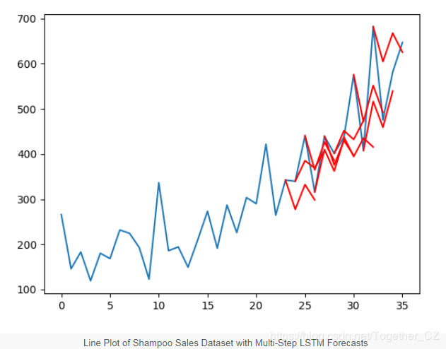
A series line plot with predictions (in red) was also created. From the graph, while the model’s skill is reasonably good, some predictions are not very good, indicating there is still much room for improvement.

Extensions

• Update LSTM. Change the example to re-fit or update the LSTM when new data is provided. 10 training epochs should be sufficient to re-train with new observations.

• Optimize LSTM. Perform a grid search on some of the LSTM parameters used in this tutorial, such as the number of epochs, number of neurons, and number of layers, to see if performance can be further improved.

• Seq2Seq. Use the encoder-decoder paradigm of LSTMs to predict each sequence and see if this offers any benefits.

• Time Horizons. Experiment with predicting different time horizons to see how the network’s behavior changes with different delivery times.

Author: Yishui Hancheng, CSDN Blog Expert, personal research areas: Machine Learning, Deep Learning, NLP, CV

Blog: http://yishuihancheng.blog.csdn.net