Skip to content

MTCNN (Multi-Task Cascaded Convolutional Networks) was proposed in 2016. As the name suggests, the algorithm adopts a cascaded CNN structure to achieve multi-task learning—face detection and face alignment, ultimately predicting the positions of face bounding boxes and landmarks.
MTCNN achieved the best results at that time (April 2016) on the FDDB, WIDER FACE, and AFLW datasets, and it was also fast (for that time), widely used in the front end of face recognition processes.
Overall, the effectiveness of MTCNN mainly benefits from the following points:
1. The cascaded CNN architecture is a coarse-to-fine process;
2. The online hard example mining (OHEM) strategy was used during training;
3. Joint face alignment learning was incorporated.
Now, let’s explore the world of MTCNN.
MTCNN’s “Promotional Poster”
MTCNN consists of three networks that together form a cascaded CNN architecture. These three networks are P-Net, R-Net, and O-Net, where the output of the former serves as the input for the latter.
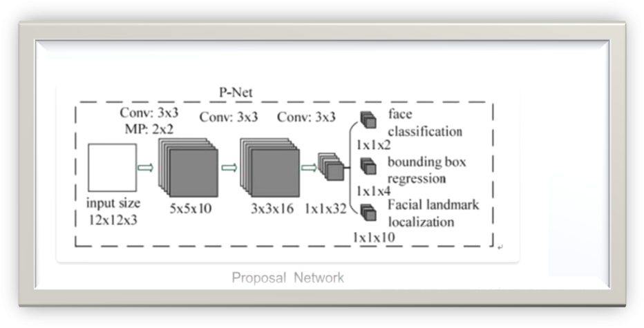
P-Net (Proposal Network)
 P-Net
As the name implies, this network is primarily used to output candidate regions containing faces. The output consists of three parts: classification results (binary classification), indicating whether it is a face, the detected face bounding box (bbox) position, and the located landmark positions.
It is important to note that the bbox and landmarks returned here are not the actual coordinate values but normalized offsets, which will be explained in detail later.
Additionally, P-Net is a Fully Convolutional Network (FCN), outputting a map with channels of 2 + 4 + 10 = 16, where 2 corresponds to the binary classification score, 4 corresponds to the offsets of the top-left and bottom-right coordinates of the bbox, and 10 corresponds to the offsets of the five landmarks (left eye, right eye, nose, left mouth corner, right mouth corner). The outputs of R-Net and O-Net will have similar meanings.
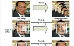
You may wonder why P-Net is designed as an FCN. From the above diagram, you can see that the input image size is 12×12, and the final output size is 1×1, which seems unnecessary. However, if you closely examine the top part of the image shown in the introduction, you should understand the reason.
P-Net
As the name implies, this network is primarily used to output candidate regions containing faces. The output consists of three parts: classification results (binary classification), indicating whether it is a face, the detected face bounding box (bbox) position, and the located landmark positions.
It is important to note that the bbox and landmarks returned here are not the actual coordinate values but normalized offsets, which will be explained in detail later.
Additionally, P-Net is a Fully Convolutional Network (FCN), outputting a map with channels of 2 + 4 + 10 = 16, where 2 corresponds to the binary classification score, 4 corresponds to the offsets of the top-left and bottom-right coordinates of the bbox, and 10 corresponds to the offsets of the five landmarks (left eye, right eye, nose, left mouth corner, right mouth corner). The outputs of R-Net and O-Net will have similar meanings.
You may wonder why P-Net is designed as an FCN. From the above diagram, you can see that the input image size is 12×12, and the final output size is 1×1, which seems unnecessary. However, if you closely examine the top part of the image shown in the introduction, you should understand the reason.
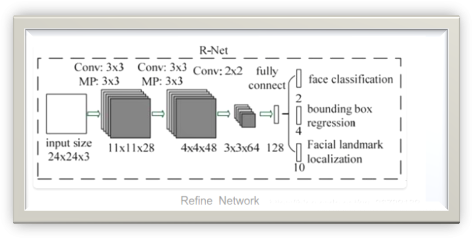 R-Net
R-Net is no longer an FCN; it uses fully connected layers at the end. Compared to P-Net, its input size and the number of channels at each layer are larger, which means its fitting results are more accurate. Its main role is to correct the results of P-Net and eliminate false positives (FP).
R-Net
R-Net is no longer an FCN; it uses fully connected layers at the end. Compared to P-Net, its input size and the number of channels at each layer are larger, which means its fitting results are more accurate. Its main role is to correct the results of P-Net and eliminate false positives (FP).
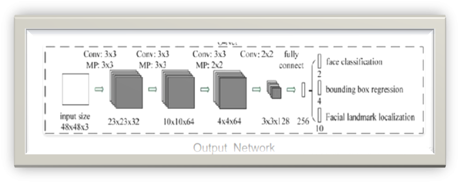
O-Net (Output Network)
 O-Net
The structure of O-Net is similar to that of P-Net, except that its input size, width, and depth are larger, allowing for more accurate final output results.
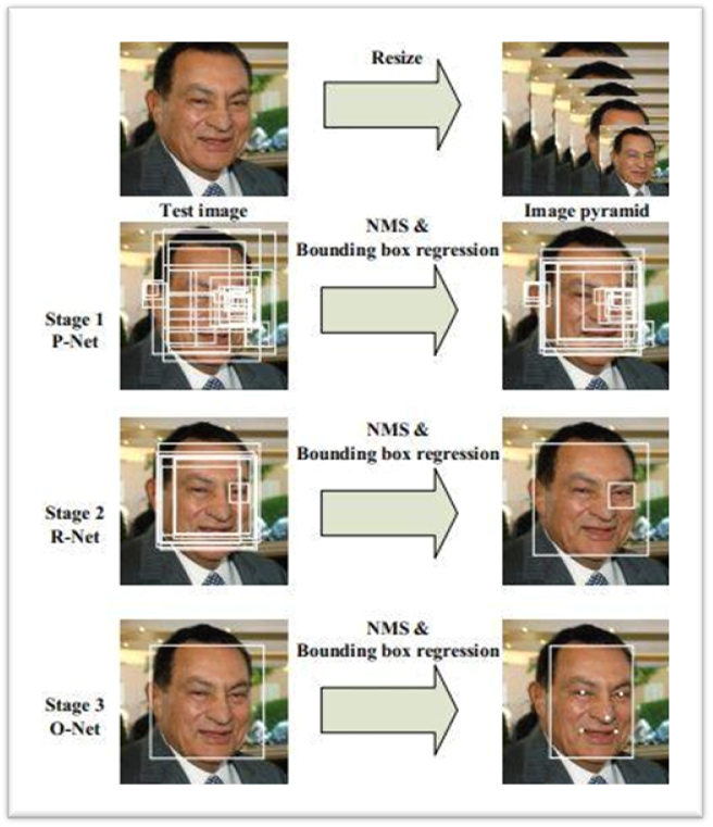
From the structure presented above, we can feel that P-Net -> R-Net -> O-Net is a coarse-to-fine process.
The inference process pipeline is as follows: process the input image to generate an image pyramid -> input to P-Net -> post-process the output of P-Net -> input to R-Net -> post-process the output of R-Net -> input to O-Net -> post-process the output of O-Net to obtain the final prediction results.
Additionally, during inference, P-Net and R-Net do not need to output the landmarks component, as the predicted face box positions are not yet accurate, making it meaningless to calculate the corresponding landmarks positions based on offsets. Ultimately, the output still depends on O-Net.
O-Net
The structure of O-Net is similar to that of P-Net, except that its input size, width, and depth are larger, allowing for more accurate final output results.
From the structure presented above, we can feel that P-Net -> R-Net -> O-Net is a coarse-to-fine process.
The inference process pipeline is as follows: process the input image to generate an image pyramid -> input to P-Net -> post-process the output of P-Net -> input to R-Net -> post-process the output of R-Net -> input to O-Net -> post-process the output of O-Net to obtain the final prediction results.
Additionally, during inference, P-Net and R-Net do not need to output the landmarks component, as the predicted face box positions are not yet accurate, making it meaningless to calculate the corresponding landmarks positions based on offsets. Ultimately, the output still depends on O-Net.
Image Pyramid
As shown in the previous section, the P-Net network architecture is trained on a single scale (12×12 size). To detect faces of different sizes, an image pyramid must be generated during inference, which is also the reason why P-Net is designed as an FCN.
First, set a minimum face size to be detected, min_size, for example, 20×20, and then set a scaling factor, typically 0.707.
Next, scale the shortest side of the image by 12 / 20, and then continuously scale the previously scaled size by the factor, for example, if the initial shortest side is s, the subsequent scales will be: s x 12 / 20, s x 12 / 20 x factor, s x 12 / 20 x factor ^2, … until s is no longer greater than 12.
Record all scales during the scaling process (while the shortest side is still greater than 12): 12 / 20, 12 / 20 x factor, 12 / 20 x factor^2, …, and finally use bilinear interpolation to scale the image at each scale to obtain the image pyramid.
Time for questions! Why is the scaling factor 0.707?
This number seems familiar, right? Yes, it is approximately equal to , but what does this represent?
Typically, in our common thinking, scaling factors are usually set to 0.5. If the side length is scaled down by 0.5, the area of the rectangle will shrink by1/4, which may miss many faces to be detected. It’s important to know that according to P-Net, each scale corresponds to one face. Therefore, we can scale the area down by 1/2 to reduce the range between scales, which means the scaling factor for the side length is
, but what does this represent?
Typically, in our common thinking, scaling factors are usually set to 0.5. If the side length is scaled down by 0.5, the area of the rectangle will shrink by1/4, which may miss many faces to be detected. It’s important to know that according to P-Net, each scale corresponds to one face. Therefore, we can scale the area down by 1/2 to reduce the range between scales, which means the scaling factor for the side length is .
The second soul-searching question in the series of “A Hundred Thousand Whys”—what impact do min_size and factor have on the inference process?
From elementary math knowledge, we know that the larger the min_size and the smaller the factor, the faster the shortest side of the image scales to near 12, thus shortening the time to generate the image pyramid. Simultaneously, the range of each scale becomes larger. Therefore, increasing min_size and decreasing factor can speed up the generation of the image pyramid, but it also increases the likelihood of missed detections.
Alright, no more questions. If I really had to ask a hundred thousand, my hands would probably be worn out.. The rest is up to you to ponder.
As mentioned above, the drawback of the image pyramid is that it is slow! It is slow because it requires continuous resizing to generate images of various sizes, and it is also slow because these images are input one by one into P-Net for detection (the output result of each image represents a candidate face region), which means multiple inference processes, which is quite scary..
.
The second soul-searching question in the series of “A Hundred Thousand Whys”—what impact do min_size and factor have on the inference process?
From elementary math knowledge, we know that the larger the min_size and the smaller the factor, the faster the shortest side of the image scales to near 12, thus shortening the time to generate the image pyramid. Simultaneously, the range of each scale becomes larger. Therefore, increasing min_size and decreasing factor can speed up the generation of the image pyramid, but it also increases the likelihood of missed detections.
Alright, no more questions. If I really had to ask a hundred thousand, my hands would probably be worn out.. The rest is up to you to ponder.
As mentioned above, the drawback of the image pyramid is that it is slow! It is slow because it requires continuous resizing to generate images of various sizes, and it is also slow because these images are input one by one into P-Net for detection (the output result of each image represents a candidate face region), which means multiple inference processes, which is quite scary..
P-Net Obtaining Candidate Face Regions
Each image of different sizes in the image pyramid is sequentially input into P-Net. For each scale of the image, a map is output, where each point of the output map has a classification score and the bbox offset for regression.
First, retain a batch of high-confidence position points, then restore each point to its corresponding face region, followed by using NMS to eliminate duplicate regions. After obtaining results retained from all scaled images, apply NMS again to remove duplicates (CW has conducted experiments showing that NMS does not work on outputs from different scales, indicating that there are no duplicates across different scales, which aligns with the idea of detecting faces of different sizes at different scales).
Finally, use the offsets obtained from regression to correct the candidate face regions to get the bbox positions.A hundred thousand why series is back—how to restore the output map point to its corresponding face region?
According to the structure design of P-Net, a point in the output feature map corresponds to a 12×12 area in the input image. Since there is a pooling layer in P-Net that performs 2x downsampling (not counting the size loss caused by the convolutional layer), we can restore the position of a point in the output feature map (x, y) as follows:
i). First restore its position in the input image: (x*2, y*2);
ii). Take this as the top-left corner of the face region, with the corresponding bottom-right corner being: (x*2 + 12, y*2 + 12);
iii). Since the image pyramid was generated with scaling, we also need to divide by the scale used at that time: (x1 = x*2 / scale, y1 = y*2 / scale), (x2 = (x*2 + 12) / scale, y2 = (y*2 + 12) / scale).
Thus, (x1, y1, x2, y2) is the restored face region corresponding to the original image.
You probably haven’t had enough, so let’s continue asking—how to calculate the face bbox position using the obtained offsets?
Using the above formulas, we can calculate the results, where x*_true and y*_true represent the positions of the face bbox, tx* and ty* represent the obtained offsets, and w and h are the width and height of the face region (x1, y1, x2, y2).
As for why this calculation works, it is determined by the labels created during training, which will be explained in the next section about the training process, so let’s hold that thought for now.
The bbox output by P-Net is not precise enough and serves merely as a candidate region containing faces, which is then corrected by R-Net.
R-Net Further Corrects Based on P-Net Results
R-Net does not directly use the output results from P-Net; it is a meticulous boy who first “gives these outputs a makeover” before using them, as follows:
i). To cover as many faces as possible, the candidate regions output by P-Net are resized into squares based on their respective long edges;
ii). Check whether the coordinates of these regions are within the original image range. Set the pixel values within the original image to the corresponding pixel values, and set others to 0;
iii). Resize the obtained image regions to 24×24 using bilinear interpolation.
After processing, all inputs are 24×24 in size, and the output post-processing is similar to P-Net: first filter a batch of high-confidence results, then use NMS to eliminate duplicates, and finally calculate the bbox positions using the offsets. The (x1,y1,x2,y2) used for offset calculation here are the bbox outputs from P-Net.
Another question arises—why not directly resize the regions within the valid range of the original image?
One way to think about it is that if the valid region is exactly the face region, there will definitely be pixel loss during resizing, resulting in loss of detail.
O-Net Detects Face and Landmark Positions
Seeing that R-Net is a meticulous boy, O-Net is also very conscious about processing the output results from R-Net in a similar manner, except that the final resize size is 48×48.
Since O-Net outputs the offsets of the landmarks, it also needs to calculate the positions of the landmarks:
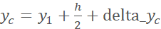
(x_true, y_true) represent the position of a landmark, tx and ty represent the corresponding offsets, and (x_box, y_box) represent the top-left position of the bbox output by R-Net, while w and h represent the width and height of the bbox.As for the calculation of bbox positions and post-processing, these are similar to what was previously described, so we will not elaborate further here.
Oh, additionally, when calculating IoU here, the denominator can be taken not as the union but as the smaller area between the current highest confidence bbox and the other bboxes. This way, the denominator becomes larger, leading to a higher IoU calculation result, which effectively lowers the NMS threshold and makes the requirements for duplicate detection more stringent.
The three networks of MTCNN are trained sequentially: first P-Net is trained, and once it is trained, its detection results are used for R-Net training data, followed by training R-Net. Similarly, after R-Net is trained, its detection results are used for O-Net training data, and finally, O-Net is trained.
Data Sample Classification
MTCNN is a multi-task architecture that integrates face detection and face alignment, usually using two datasets for training. One dataset trains for face detection, and the other trains for face alignment (which can also train for face detection).
When processing training data, random cropping is applied to the images, and the specific method will be explained later. The training samples can be divided into four categories:
i). Positive: Cropped images with IoU >= 0.65 with the face annotation box, category label is 1;
ii). Part: Cropped images with IoU [0.4, 0.65), category label is -1;
iii). Negative: Cropped images with IoU < 0.3 with the face annotation box, category label is 0;
iv). Landmarks: Samples from the dataset for training face alignment, category label is -2.
Classification loss is calculated using Positive and Negative samples, bbox regression loss is calculated using Positive and Part samples, and only Landmarks samples are used to calculate landmarks regression loss.
Time for a hundred thousand whys—why only use Positive and Negative to calculate classification loss?
This is likely because these positive and negative samples have a significant difference in IoU with the annotation box, making them easier to distinguish, thus facilitating model convergence.
[0.4, 0.65), category label is -1;
iii). Negative: Cropped images with IoU < 0.3 with the face annotation box, category label is 0;
iv). Landmarks: Samples from the dataset for training face alignment, category label is -2.
Classification loss is calculated using Positive and Negative samples, bbox regression loss is calculated using Positive and Part samples, and only Landmarks samples are used to calculate landmarks regression loss.
Time for a hundred thousand whys—why only use Positive and Negative to calculate classification loss?
This is likely because these positive and negative samples have a significant difference in IoU with the annotation box, making them easier to distinguish, thus facilitating model convergence.
Label Creation
Time to fill in the gaps! The two gaps previously mentioned will be filled here, so pay attention!
The label processing for P-Net, R-Net, and O-Net has some differences, which will be introduced one by one below.
P-Net
Negative Samples
1. Randomly crop the image, resulting in a square with side length s=(12, min(H, W)), where H and W are the height and width of the image, respectively. Move the top-left corner of the image downward to the bottom-right, resulting in new coordinates
 (0, W – s),
 (0, H – s), thus the bottom-right coordinates of the cropped image are (x2=x1 + s, y2=y1 + s).
2. Calculate the IoU between the cropped image and all annotation boxes in the original image. If the maximum IoU < 0.3, the cropped image is considered a negative sample. Resize it to 12×12, and the corresponding category label is set to 0, saved for training.
3. Repeat steps 1 and 2 until 50 negative sample images are generated.
4. For each annotation box in the image, repeat random cropping 5 times to generate negative samples. The cropped image’s side length s is the same as in step 1, moving the left-top corner of the bbox (x1, y1), with new coordinates being (nx1=x1 + delta_x, ny1=y1 + delta_y), where delta_x
(0, H – s), thus the bottom-right coordinates of the cropped image are (x2=x1 + s, y2=y1 + s).
2. Calculate the IoU between the cropped image and all annotation boxes in the original image. If the maximum IoU < 0.3, the cropped image is considered a negative sample. Resize it to 12×12, and the corresponding category label is set to 0, saved for training.
3. Repeat steps 1 and 2 until 50 negative sample images are generated.
4. For each annotation box in the image, repeat random cropping 5 times to generate negative samples. The cropped image’s side length s is the same as in step 1, moving the left-top corner of the bbox (x1, y1), with new coordinates being (nx1=x1 + delta_x, ny1=y1 + delta_y), where delta_x [max(-s, -x1), w), delta_y
 [max(-s, -y1), h), meaning the top-left corner of the annotation box is randomly moved up, down, left, or right, resulting in new coordinates for the bottom-right corner (nx2=nx1 + s, ny2=ny1 + s). If the bottom-right corner exceeds the original image range, discard the cropped image and proceed to the next cropping.
Positive and Part Samples
5. Immediately after step 4, repeat random cropping 20 times to generate Positive and Part samples.
The cropped image’s side length s

 is between 0.8 times the short side of the bbox and 1.25 times the long side.
Randomly move the center point of the bbox up, down, left, or right, with movement ranges delta_
is between 0.8 times the short side of the bbox and 1.25 times the long side.
Randomly move the center point of the bbox up, down, left, or right, with movement ranges delta_ [-0.2w, 0.2w), delta_
 [-0.2h, 0.2h), leading to new center point coordinates
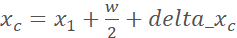 ,
,  accordingly:
The top-left and bottom-right coordinates are
accordingly:
The top-left and bottom-right coordinates are ,
(
,
( ) If the bottom-right corner exceeds the original image range, discard the result of this cropping and continue with the next random cropping.
6. If the cropped image has IoU >= 0.65 with the bbox, it is considered a positive sample and resized to 12×12, with the category label set to 1; otherwise, if IoU >= 0.4, it is considered a part sample, also resized to 12×12, with the category label set to -1;
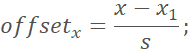
7. For the Positive and Part samples, calculate the offsets for the top-left and bottom-right of the bbox:
where (x, y) are the coordinates of the top-left/bottom-right of the annotation box, (nx, ny) are the coordinates of the top-left/bottom-right of the cropped image, and s is the side length. This means the normalized displacement of the two corners of the annotation box relative to the corresponding corners of the cropped image. Finally, save the cropped images, category labels, and offset labels for training.
) If the bottom-right corner exceeds the original image range, discard the result of this cropping and continue with the next random cropping.
6. If the cropped image has IoU >= 0.65 with the bbox, it is considered a positive sample and resized to 12×12, with the category label set to 1; otherwise, if IoU >= 0.4, it is considered a part sample, also resized to 12×12, with the category label set to -1;
7. For the Positive and Part samples, calculate the offsets for the top-left and bottom-right of the bbox:
where (x, y) are the coordinates of the top-left/bottom-right of the annotation box, (nx, ny) are the coordinates of the top-left/bottom-right of the cropped image, and s is the side length. This means the normalized displacement of the two corners of the annotation box relative to the corresponding corners of the cropped image. Finally, save the cropped images, category labels, and offset labels for training.
Landmarks Samples
8. Landmarks samples are processed separately in another dataset, where each image contains a single face. For each image, repeat random cropping 10 times, using the same method as for generating Positive and Part samples. If the bottom-right coordinates of the cropped image are not within the original image range or if the IoU with the annotation box is < 0.65, discard this cropping result and proceed to the next.
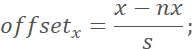
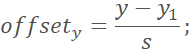
9. Calculate the bbox and landmarks offset labels, where the calculation method for the bbox is the same as for Positive and Part; the landmarks offsets are calculated as follows:
 where (x, y) are the coordinates of the annotated landmark,
 is the top-left corner of the cropped image, and s is the side length of the cropped image, which is the normalized displacement of the annotated landmark relative to the top-left corner of the cropped image.
R-Net
Before creating the labels for R-Net, the trained P-Net dataset is used for detection, and the subsequent data processing is similar to that of P-Net, which will be introduced below.
1. Use the trained P-Net to detect the images in the dataset, saving the original images, annotations, and detected bbox positions accordingly.
2. Extract the original image, annotations, and detected bbox one by one. For each bbox, if its size is less than 20 (min_size, representing the minimum face size to be detected) or if the coordinates are not within the original image range, discard the detected bbox and continue to the next; otherwise, crop the corresponding area from the original image and resize it to 24×24 for later use.
Negative Samples
3. Calculate the IoU between the bbox and all annotation boxes. If the maximum IoU < 0.3 and the current number of generated negative samples is less than 60, consider the cropped image as a negative sample, category label is 0, saved for training.
Positive and Part Samples
4. Otherwise, if the maximum IoU >= 0.65 or 0.4 <= maximum IoU < 0.65, label the cropped image as a Positive sample or Part sample, respectively, with category labels of 1 or -1. Also, extract the annotation box corresponding to the maximum IoU for offset calculation, using the same method as mentioned in P-Net, and finally save the cropped image, category label, and offset label for training.
O-Net
Before creating the labels for O-Net, the trained P-Net and R-Net are used for detection, and then the R-Net predicted bbox and the corresponding original images and annotations are saved for O-Net use.
The label creation process is almost the same as R-Net’s, except there is no minimum negative sample quantity limit (P-Net has 50, R-Net has 60). Additionally, if the longest side of the annotation box in the landmarks dataset is less than 40 or the coordinates are not within the original image range, this sample will be discarded.
Loss Function
The loss consists of three parts: classification loss, bbox regression loss, and landmarks regression loss.
Each network’s loss is weighted by these three losses, where classification loss uses cross-entropy loss, and regression losses use L2 distance loss.
In the formula, j represents different tasks (classification, bbox regression, landmarks regression),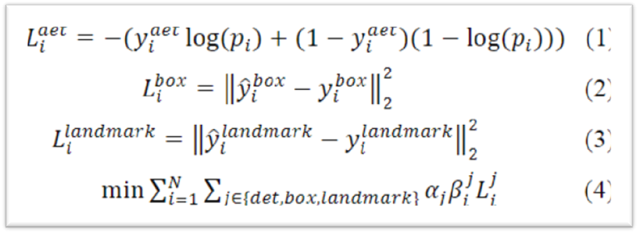 indicates the loss weight for different tasks. For P-Net and R-Net, the weights for their classification loss, bbox regression loss, and landmarks regression loss are 1:0.5:0.5, while in O-Net, they are 1:0.5:1.
 is whether the i-th sample contributes to the loss in task j; it is 1 if it does, otherwise 0. For example, for Negative samples, thisβ value would be 0.
OHEM (Online Hard Example Mining)
The online hard example mining strategy is only used when calculating classification loss. To put it simply, it selects the top 70% of samples with the highest loss as hard samples, and during backpropagation, only the loss from these 70% of hard samples is used. The author’s experiments in the paper show that this approach can bring a 1.5-point performance improvement on the FDDB dataset.
Finally, let’s summarize the entire pipeline of MTCNN:
First, generate an image pyramid for the image to be detected, input it into P-Net, obtain the output, and filter out candidate face regions using classification confidence and NMS;
Then, based on these candidate regions, crop the corresponding images from the original image, input them into R-Net, obtain the output, and similarly use classification confidence and NMS to filter out false positives, resulting in a more accurate batch of candidates;
Finally, based on this batch of candidates, crop the corresponding images from the original image, input them into O-Net, and output the final predicted bbox and landmark positions.