Author: Justin Ho

Editor: Xixiaoyao’s Cute Shop Source: https://zhuanlan.zhihu.com/p/28749411

Introduction

The CNN has evolved from AlexNet in 2012 to various CNN models invented by scientists, each deeper, more accurate, and lighter than the last. Below, we will briefly review some revolutionary works in recent years and explore the future direction of CNN transformations from these innovative works.

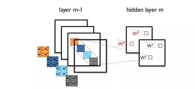
Can Convolution Only Be Done in the Same Group?

Group convolution first appeared in AlexNet. Due to limited hardware resources at the time, the convolution operations could not all be processed on the same GPU during the training of AlexNet, so the author divided the feature maps among multiple GPUs for processing, and finally fused the results from multiple GPUs.

The concept of group convolution has far-reaching implications. Currently, some lightweight SOTA (State Of The Art) networks utilize group convolution operations to save computation. However, the question arises: if group convolution is distributed across different GPUs, the computation for each GPU is reduced to 1/groups. But if it is still computed on the same GPU, does the overall computation remain unchanged? I found an introduction to group convolution operations on PyTorch, hoping readers can help answer my question.

Regarding this issue, a Zhihu user friend @Cai Guanyu offered his insights: https://www.zhihu.com/people/cai-guan-yu-62/activities

I feel that group convolution itself should greatly reduce the parameters. For example, when the input channel is 256 and the output channel is also 256, with a kernel size of 3*3, if we do not use group convolution, the parameters would be 256*3*3*256. If the group is 8, each group’s input and output channels would be 32, resulting in parameters of 8*32*3*3*32, which is one-eighth of the original. This is my understanding.

My understanding is that the output feature maps of each group from group convolution should be combined in a concatenate manner rather than element-wise add, so the output channel of each group is input channels / #groups, significantly reducing the number of parameters.

Is a Larger Convolution Kernel Always Better?

AlexNet used some very large convolution kernels, such as 11×11 and 5×5. Previously, the belief was that the larger the convolution kernel, the larger the receptive field (感受野), allowing more image information to be captured, thus resulting in better features. However, large convolution kernels lead to a significant increase in computation, which is detrimental to increasing model depth and reduces computational performance. Therefore, in VGG (the first to use it) and Inception networks, the combination of two 3×3 convolution kernels proved to be more effective than one 5×5 convolution kernel, while also reducing the number of parameters (3×3×2+1 VS 5×5×1+1). As a result, 3×3 convolution kernels have been widely used in various models.

Must Each Layer’s Convolution Kernel Size Be the Same?

Traditional stacked networks typically use a single size of convolution kernel for each layer, such as the VGG structure, which uses a large number of 3×3 convolution layers. In fact, multiple convolution kernels of different sizes can be used in the same feature map layer to capture features at different scales, and combining these features often yields better results than using a single convolution kernel. Google’s GoogleNet, or the Inception series of networks, employs a structure with multiple convolution kernels:

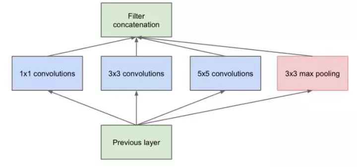
As shown in the figure above, an input feature map is processed simultaneously by 1×1, 3×3, and 5×5 convolution kernels, and the resulting features are combined to obtain better features. However, this structure poses a serious problem: the number of parameters is significantly larger than that of a single convolution kernel, and such a large computational load can lead to inefficiency in the model. This leads to the introduction of a new structure.

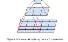
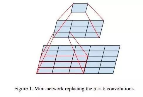
How Can We Reduce the Number of Parameters in Convolutional Layers?

The team that invented GoogleNet found that simply introducing multiple sizes of convolution kernels would result in a large number of additional parameters. Inspired by the 1×1 convolution kernel in Network In Network, to solve this problem, they added some 1×1 convolution kernels to the Inception structure, as illustrated:

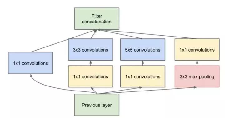
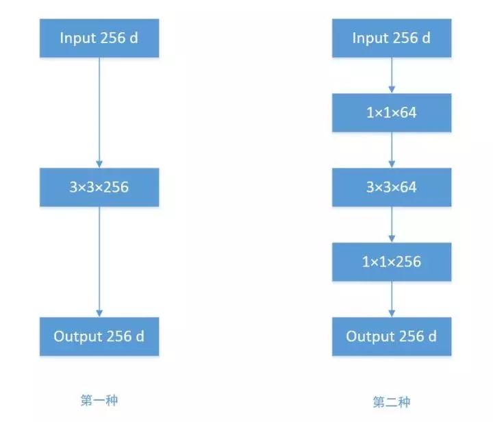
According to the figure above, let’s do a comparative calculation. Assuming the input feature map dimension is 256 and the output dimension is also 256, we have the following two operations:

(1) The 256-dimensional input directly goes through a 3×3×256 convolution layer, producing a 256-dimensional feature map, resulting in a parameter count of: 256×3×3×256 = 589,824

(2) The 256-dimensional input first goes through a 1×1×64 convolution layer, then a 3×3×64 convolution layer, and finally a 1×1×256 convolution layer, outputting 256 dimensions, with a parameter count of: 256×1×1×64 + 64×3×3×64 + 64×1×1×256 = 69,632. This reduces the parameter count of the first operation to one-ninth!

The 1×1 convolution kernel is also considered a profoundly influential operation, and in the future, large networks will apply the 1×1 convolution kernel to reduce the number of parameters.

Is a Deeper Network Harder to Train?

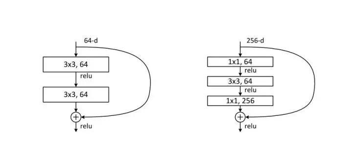
Traditional stacked convolutional networks encounter a problem: as the number of layers increases, the performance of the network deteriorates. This is largely due to the increasing severity of gradient vanishing as layers deepen, making it difficult to train the shallower layers through backpropagation. To solve this problem, the great Kai-Ming He proposed a “residual network” that facilitates the gradient flow to the shallower layers, and this “skip connection” provides additional benefits. For further reference, see the PPT “Extremely Deep Networks (ResNet/DenseNet): Why Skip Connections Are Effective and More” [1], as well as my article: Why ResNet and DenseNet Can Be So Deep? A Detailed Explanation of Why Residual Blocks Can Solve the Gradient Vanishing Problem [2], and consider the comments below for further thought.

Must We Consider Both Channels and Regions When Convolving?

The standard convolution process can be seen in the figure above, where a 2×2 convolution kernel considers all channels in the corresponding image region simultaneously. However, the question arises: why must we consider both the image region and the channels simultaneously? Why can’t we consider the channels and spatial regions separately?

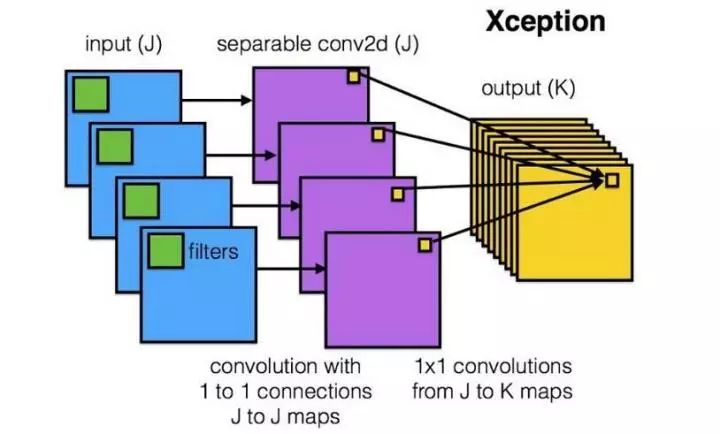
The Xception network was invented based on the above questions. We first perform convolution operations on each channel separately, with as many filters as there are channels. After obtaining the new channel feature maps, we then perform standard 1×1 cross-channel convolution on these new channel feature maps. This operation is called “DepthWise convolution”, abbreviated as “DW”.

This operation is quite effective, having surpassed the performance of InceptionV3 in the ImageNet 1000-class classification task while also significantly reducing the number of parameters. Let’s calculate it: assuming the input channel number is 3 and the required output channel number is 256, we have two approaches:

1. Directly connect a 3×3×256 convolution kernel, resulting in a parameter count of: 3×3×3×256 = 6,912

2. DW operation, completed in two steps, resulting in a parameter count of: 3×3×3 + 3×1×1×256 = 795, again reducing the parameter count to one-ninth!

Therefore, a depthwise operation significantly reduces the number of parameters compared to standard convolution operations, and the paper indicates that this model achieves better classification results.

Within 12 hours of publishing this article, a netizen privately messaged me, introducing the historical work behind Depthwise and Pointwise, and Xception and Mobilenet also cite their 2016 work, namely Min Wang et al’s Factorized Convolutional Neural Networks. In this paper, the Depthwise of each channel output feature map (referred to as “base layer”) can have more than one, while in Xception, the Depthwise separable Convolution is precisely the case of “single base layer.” I recommend interested readers to pay attention to their work; here is a blog post introduction: [Deep Learning] Speeding Up Convolutional Layers with Factorized Convolutional Neural Networks. The earliest introduction to separable convolution, as mentioned by the Xception authors, should trace back to Laurent Sifre’s 2014 work, Rigid-Motion Scattering For Image Classification, section 6.2.

Can Group Convolution Randomly Group Channels?

In AlexNet’s Group Convolution, the channels of features are evenly divided into different groups, and finally, two fully connected layers are used to fuse features. This way, different groups’ features can only be fused at the last moment, which is quite detrimental to the model’s generalization. To solve this problem, ShuffleNet performs a channel shuffle before each stacking of this Group conv layer, and the shuffled channels are assigned to different groups. After performing one group conv, another channel shuffle is performed, and then assigned to the next layer of group convolution, and this process continues.

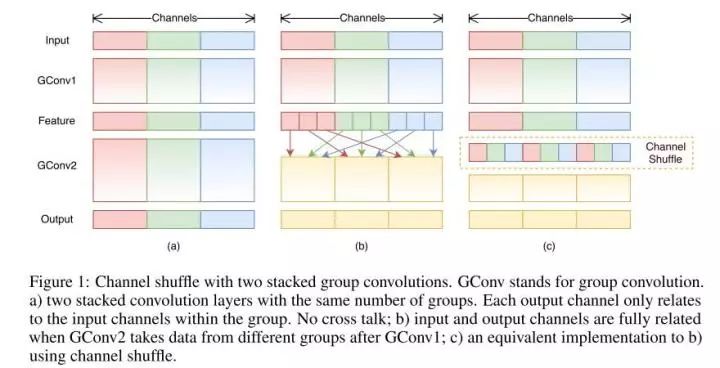
After channel shuffling, the features output by Group conv can consider more channels, and the representativeness of the output features naturally increases. Additionally, AlexNet’s group convolution is essentially standard convolution, while the group convolution operation in ShuffleNet is depthwise convolution. Therefore, by combining channel shuffling and group depthwise convolution, ShuffleNet can achieve an extremely low number of parameters and accuracy comparable to AlexNet, even surpassing Mobilenet!

Additionally, it is worth mentioning that Microsoft Research Asia (MSRA) has recently conducted similar work, proposing an IGC unit (Interleaved Group Convolution), which performs two group convolutions in a manner similar to that of ShuffleNet. The Xception module can be seen as a special case of interleaved group convolution. I highly recommend reading this paper: Wang Jingdong’s Detailed Explanation of ICCV 2017 Selected Paper: Interleaved Group Convolution for General Convolutional Neural Networks.

It is important to note that Group conv is a method of channel grouping, whereas Depthwise + Pointwise refers to convolution methods. ShuffleNet simply applies both methods together. Thus, Group conv and Depthwise + Pointwise are not equivalent.

Are Features Between Channels Equal?

In Inception, DenseNet, or ShuffleNet, the features generated from all channels are combined without weighting. So why assume that the features from all channels have equal contributions to the model? This is a good question, leading to the emergence of the ImageNet 2017 champion SENet.

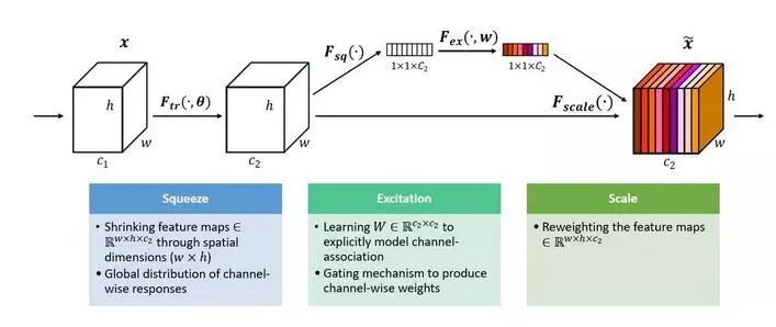
A set of features output from the previous layer is split into two routes: the first route passes directly, while the second first undergoes a Squeeze operation (Global Average Pooling), compressing each channel’s 2D features into a 1D feature channel vector (each number represents the corresponding channel’s feature). This is followed by an Excitation operation, where this feature channel vector is input into two fully connected layers with a sigmoid, modeling the correlation between feature channels. The output represents the weight corresponding to each channel, which is then multiplied by the original features (first route) to complete the weight distribution of feature channels.

Let Convolution Kernels See a Larger Area

A standard 3×3 convolution kernel can only see a corresponding area of 3×3 in size. However, to allow the convolution kernel to see a larger area, dilated convolution makes this possible. The structure in the original paper on dilated convolution is illustrated in the following figure:

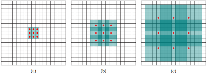
In the above figure, the convolution kernel size remains 3×3, but there is a hole between each convolution point, meaning that only 9 red points in the green 7×7 area are processed by convolution, while the weights of the other points are 0. Thus, even though the convolution kernel size remains unchanged, it can now see a larger area. For a detailed explanation, please refer to this answer: How to Understand Dilated Convolution?

Must Convolution Kernels Be Rectangular?

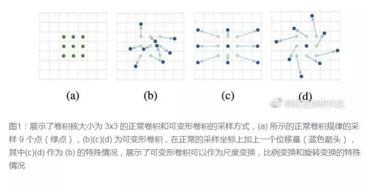
Traditional convolution kernels are generally rectangular or square, but MSRA has proposed a rather counterintuitive insight: the shape of the convolution kernel can vary. Deformable convolution kernels can focus only on the regions of interest in the image, resulting in better feature recognition.

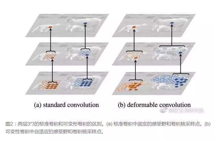
To achieve this, one can simply add a filtering layer in front of the original filter, where this layer learns the position offsets of the next convolution kernel. This only adds one filtering layer, or one can directly use a certain layer’s filter in the original network as the filter for learning the offsets, thus the actual increase in computational load is quite small, but it allows for deformable convolution kernels, resulting in better feature recognition. For a detailed interpretation from MSRA, please refer to this link: Deformable Convolutional Networks: A New “Vision” for Computers.

Inspiration and Reflection

More and more CNN models are evolving from giant networks to lightweight networks, with model accuracy increasing. The industry focus is no longer on improving accuracy (as it is already quite high) but on the trade-off between speed and accuracy, hoping for models that are both fast and accurate. Thus, from the original AlexNet and VGGnet, to the smaller Inception and ResNet series, to the currently deployable mobilenet and ShuffleNet (reducing to 0.5mb!), we can observe several trends:

Regarding Convolution Kernels:

• Large convolution kernels are replaced with multiple small convolution kernels;
• Single-size convolution kernels are replaced with multi-size convolution kernels;
• Fixed-shape convolution kernels tend to use deformable convolution kernels;
• 1×1 convolution kernels (bottleneck structures) are utilized.

Regarding Convolution Layer Channels:

• Standard convolution is replaced with depthwise convolution;
• Group convolution is utilized;
• Channel shuffle is performed before group convolution;
• Channel-weighted calculations are applied.

Regarding Convolution Layer Connections:

• Skip connections are used to deepen models;
• Densely connected structures are employed, allowing each layer to fuse outputs from other layers (DenseNet).

Inspiration

Analogous to the channel weighting operation, can convolution layer cross-layer connections also undergo weighted processing? Will the combination of bottleneck + group conv + channel shuffle + depthwise become the standard configuration for reducing parameters in the future?

Important! The Pytorch group for Natural Language Processing has been established. We have organized the official Pytorch tutorial in Chinese. Add the assistant to receive it and also join the official group! Note: Please modify the remark to [School/Company + Name + Direction] when adding. For example —— Harbin Institute of Technology + Zhang San + Dialogue System. The account owner, please avoid adding if you are a micro merchant. Thank you!

Recommended Reading:
NLP Learning (1) — Introduction to NER

NLP Learning (2) — Overview of NER

Softmax Function and Cross-Entropy