Comprehensive Summary of Optimization Algorithms in Machine Learning

Source: Internet

Introduction

For almost all machine learning algorithms, whether supervised learning, unsupervised learning, or reinforcement learning, the ultimate goal generally boils down to solving optimization problems. Therefore, optimization methods play a central role in the derivation and implementation of machine learning algorithms. In this article, the author will provide a comprehensive summary of the optimization algorithms used in machine learning and clarify their direct relationships, helping you understand this part of knowledge from a global perspective.

Mathematical Models Required by Machine Learning

Almost all machine learning algorithms ultimately seek the extreme value of an objective function, that is, an optimization problem. For example, in supervised learning, we need to find the best mapping function f(x) that minimizes the loss function for training samples (minimizing empirical risk or structural risk):

Comprehensive Summary of Optimization Algorithms in Machine Learning

Here, N is the number of training samples, L is the loss function for a single sample, w is the model parameters to be solved, which are the parameters of the mapping function, xi is the feature vector of the sample, and yi is the label value of the sample.

Or find an optimal probability density function p(x) that maximizes the log-likelihood function for training samples (maximum likelihood estimation):

Here, θ are the model parameters to be solved, which are the parameters of the probability density function.

For unsupervised learning, take clustering algorithms as an example, the algorithm needs to minimize the sum of distances from each sample in the class to the class center:

Here, k is the number of types, x is the sample vector, μi is the class center vector, and Si is the sample set of the i-th class.

For reinforcement learning, we need to find an optimal policy, that is, a mapping function from state s to action a (deterministic policy; for non-deterministic policy, it is the probability of executing each action):

So that given any state, the cumulative reward obtained after executing the action a determined by this policy function is maximized:

Here, the state value function is used.

Overall, the core goal of machine learning is to provide a model (generally a mapping function), then define an evaluation function (objective function) for the quality of this model, and solve the maximum or minimum of the objective function to determine the parameters of the model to obtain the desired model. In these three key steps, the first two are the problems that machine learning needs to study, establishing a mathematical model. The third problem is a pure mathematical problem, namely optimization methods, which is the core of this article.

Classification of Optimization Algorithms

For optimization objective functions of various machine learning algorithms with different forms and characteristics, we have found various solving algorithms suitable for them. Except for a few problems that can be solved optimally by brute force search, we divide the optimization algorithms used in machine learning into two types (this article does not consider stochastic optimization algorithms such as simulated annealing, genetic algorithms, etc.):

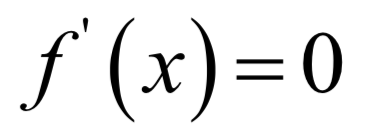
Analytical Solution
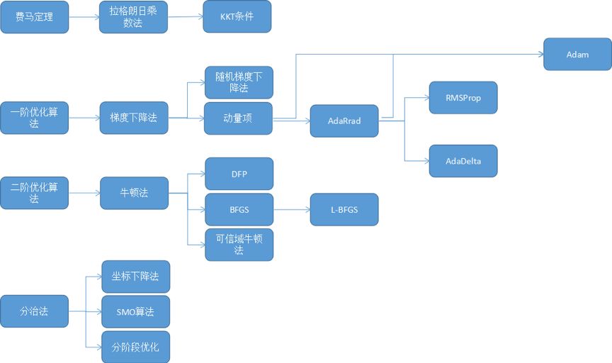
Numerical Optimization

The former provides an exact analytical solution to an optimization problem, generally a theoretical result. The latter is used to approximate the optimal point when it is very difficult to provide an exact calculation formula for the extreme point. In addition, there are other solving ideas, such as divide and conquer, dynamic programming, etc. A good optimization algorithm needs to meet:

Can correctly find extreme points in various situations
Fast speed

The following figure illustrates the classification of these algorithms and their relationships:

Next, we will elaborate according to this diagram.

Fermat’s Theorem

For a differentiable function, the unified method for finding its extreme value is to find the point where the derivative equals 0, which is Fermat’s theorem. This theorem in calculus states that for a differentiable function, the derivative must be 0 at the extreme point:

For multivariable functions, the gradient must equal 0:

Points where the derivative equals 0 are called stationary points. It is important to note that the derivative being 0 is only a necessary condition for the function to reach an extreme value, not a sufficient condition; it is merely a suspected extreme point. Whether it is an extreme value, whether it is a maximum or minimum, needs to be determined by higher-order derivatives. For a univariate function, assuming x is a stationary point:

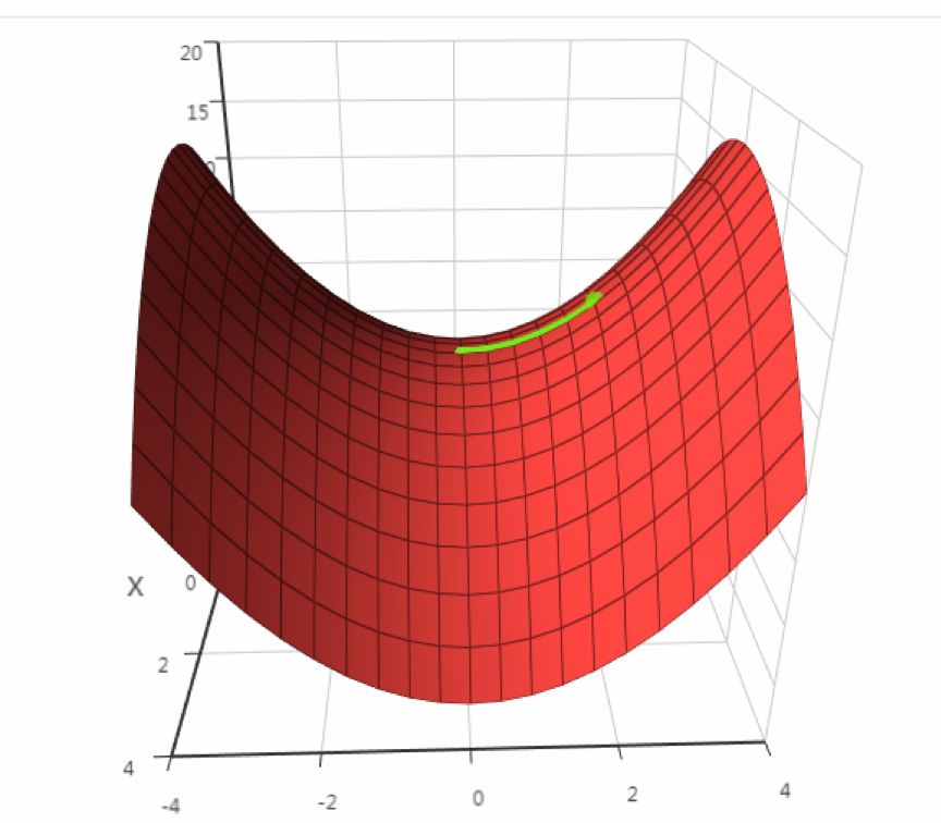
If f”(x) > 0, then it is a minimum at that point
If f”(x) < 0, then it is a maximum at that point
If f”(x) >= 0, further examination of higher-order derivatives is needed

For multivariable functions, assuming x is a stationary point:

If the Hessian matrix is positive definite, the function has a minimum at that point
If the Hessian matrix is negative definite, the function has a maximum at that point
If the Hessian matrix is indefinite, further examination is needed (this part is incorrect)

At points where the derivative equals 0, the function may not take extreme values; this is called a saddle point. The following figure is an example of a saddle point (from SIGAI Cloud Laboratory):

In addition to saddle points, optimization algorithms may also encounter another problem: the local extreme value problem, where a stationary point is an extreme point but not a global extreme point. If we impose constraints on the optimization problem, we can effectively avoid these two issues. A typical case is convex optimization, which requires the feasible region of the optimization variable to be a convex set, and the objective function to be a convex function.

Although stationary points are only a necessary condition for the function to achieve an extreme value and not a sufficient condition, if we find stationary points, it is much easier to determine and filter whether they are extreme points. Whether for theoretical results or numerical optimization algorithms, generally, finding stationary points is the goal of finding extreme points. For univariate functions, we first take the derivative, then solve the equation where the derivative equals 0 to find all stationary points. For multivariable functions, we take the partial derivative with respect to each variable, set them to 0, and solve the system of equations to reach all stationary points. These are the basic methods taught in calculus. Fortunately, in machine learning, many objective functions are differentiable, so we can use this method.

Lagrange Multiplier Method

Fermat’s theorem provides the necessary condition for the extreme value of functions without constraints. For some practical application problems, there are usually equality or inequality constraints. The classical solution for extreme value problems with equality constraints is the Lagrange multiplier method.

For the following problem:

Construct the Lagrange multiplier function:

At the optimal point, the derivatives with respect to x and the multiplier variables λi must both equal 0:

Solving this equation gives the optimal solution. For a more detailed explanation of the Lagrange multiplier method, you can read any advanced mathematics textbook. The places where the Lagrange multiplier method is used in machine learning include:

Principal Component Analysis
Linear Discriminant Analysis
Laplacian Eigenmaps in Manifold Learning
Hidden Markov Model

KKT Conditions

The KKT conditions are a generalization of the Lagrange multiplier method, used to solve functions with both equality and inequality constraints. For the following optimization problem:

Similar to the Lagrange dual approach, the KKT conditions construct the following multiplier function:

λ and μ are called KKT multipliers. At the optimal solution, x* should satisfy the following conditions:

The equality constraint hj(x*)=0 and the inequality constraint gk(x*)<=0 should be satisfied, and ▽xL(x*)=0, just like the previous Lagrange multiplier method. The only additional condition is regarding gi(x):

The KKT conditions are only necessary conditions for achieving extreme values, not sufficient conditions. The places where KKT conditions are used in machine learning include:

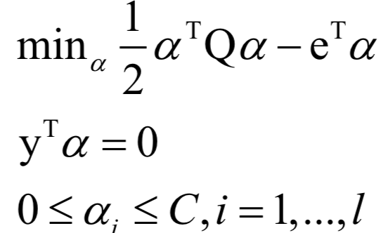
Support Vector Machine (SVM)

Numerical Optimization Algorithms

The three methods described earlier can be used in theoretical derivations and in cases where specific formulas for solving equations can be obtained (such as linear functions, maximum likelihood estimation for normal distributions). However, for the vast majority of functions, the equations where the gradient equals 0 cannot be directly solved, such as equations containing transcendental functions like exponential functions and logarithmic functions. For such unsolvable equations, we can only use approximate algorithms to solve them, that is, numerical optimization algorithms. These numerical optimization algorithms generally utilize the derivative information of the objective function, such as first-order and second-order derivatives. If first-order derivatives are used, they are called first-order optimization algorithms. If second-order derivatives are used, they are called second-order optimization algorithms.

In engineering implementation, iterative methods are usually used, starting from an initial point x0, repeatedly using a certain rule to move from xk to the next point xk+1, constructing such a sequence until convergence to the point where the gradient equals 0. That is, the following limit holds:

These rules generally utilize first-order derivative information, i.e., the gradient; or second-order derivative information, i.e., the Hessian matrix. Thus, the core of the iterative method is to obtain an iterative formula determined by the previous point to determine the next point:

Gradient Descent Method

The gradient descent method searches in the direction opposite to the gradient, utilizing the first-order derivative information of the function. The iterative formula for the gradient descent method is:

According to the first-order Taylor expansion of the function, in the negative gradient direction, the function value decreases. As long as the learning rate is set small enough and does not reach the point where the gradient equals 0, the function value will decrease in each iteration. The reason for setting the learning rate to a very small positive number is to ensure that the value xk+1 after the iteration is within the neighborhood of the previous value xk, thus allowing us to ignore the higher-order terms in the Taylor expansion and ensure that the function value decreases during iteration.

The gradient descent method and its variants are widely used in machine learning, especially in deep learning.

Momentum Term

To speed up the convergence of the gradient descent method and reduce oscillations, a momentum term is introduced. The parameter update formula after adding this term is:

Where Vt+1 is the momentum term, which replaces the previous gradient term. The calculation formula for the momentum term is:

It is the weighted average of the previous momentum term and the current gradient value, where α is the learning rate and μ is the momentum term coefficient. If expanded according to time t, then in the t-th iteration, all gradient values from the first to t-th iterations are used, and the old gradient values decay exponentially with the coefficient μt:

The momentum term accumulates the previous gradient values during iterations, allowing the current iteration to move forward in the direction of previous inertia.

AdaGrad Algorithm

AdaGrad is the most direct improvement of the gradient descent method. The gradient descent method relies on a manually set learning rate; if it is set too small, convergence is too slow, and if it is set too large, it may lead to non-convergence of the algorithm. Setting an appropriate value for this learning rate is very difficult.

The AdaGrad algorithm dynamically adjusts the learning rate based on historical gradient values from previous iterations, and each component xi of the optimization variable vector X has its own learning rate. The parameter update formula is:

Where α is the learning factor, gt is the gradient vector of the parameters at the t-th iteration, ε is a small positive number to avoid division by zero, and the subscript i indicates the component of the vector. The only difference from the standard gradient descent method is the additional term in the denominator, which accumulates the historical gradient values up to this iteration to generate the coefficient for gradient descent. According to this formula, the absolute value of historical derivative values determines the size of the component learning rate; the larger the historical derivative value, the smaller the component learning rate, and vice versa. Although it has achieved adaptive learning rates, this algorithm still has problems: a global learning rate α needs to be manually set, and as time accumulates, the denominator in the formula gets larger, causing the learning rate to approach 0, making it impossible to effectively update parameters.

RMSProp Algorithm

The RMSProp algorithm is an improvement over AdaGrad, avoiding the problem of the learning rate approaching 0 due to long-term accumulation of gradient values. The specific approach is to construct a vector RMS from gradient values, initialized to 0, which accumulates the historical squared gradient values according to a decay coefficient. The update formula is:

AdaGrad directly accumulates all historical squared gradients, while here the historical squared gradient values are accumulated after decaying with δt. The parameter update formula is:

Where δ is a manually set parameter, and like AdaGrad, a global learning rate α also needs to be manually specified.

AdaDelta Algorithm

AdaDelta is also an improvement over AdaGrad, avoiding the problem of the learning rate approaching 0 due to long-term accumulation of gradient values, and it also removes the dependence on a manually set global learning rate. Assuming the parameter to be optimized is x, the gradient value of the parameter at the t-th iteration calculated by the gradient descent method is gt. The algorithm first initializes the following two vectors to zero:

Where E[g2] is the accumulated value of the squared gradient (calculated separately for each component), the update formula is:

Here, g2 is the square of each element of the vector, and all subsequent calculation formulas are performed for each component of the vector. Next, calculate the following RMS quantity:

This is also a vector, calculated separately for each component of the vector. Then calculate the update value of the parameter:

The calculation formula for RMS[Δx]t-1 is similar to this. This update value is also constructed through gradients, except that the learning rate is determined by historical gradient values. The update formula is:

The iterative formula for parameter updates is:

Adam Algorithm

The Adam algorithm integrates adaptive learning rates with momentum terms. The algorithm constructs two vectors m and v from the gradient; the former is the momentum term, and the latter accumulates the squared gradient sum to construct the adaptive learning rate. Their initial values are 0, and the update formula is:

Where β1, β2 are manually specified parameters, and i is the index of the vector component. Relying on these two values constructs the update value for the parameters, and the parameter update formula is:

Here, m is similar to the momentum term, and v is used to construct the learning rate.

Stochastic Gradient Descent Method

Assuming the training sample set has N samples, the goal of supervised learning algorithms during training is the average loss function over this dataset:

Where L(w,xi,yi) is the loss function for a single training sample (xi,yi), w is the parameters to be learned, r(w) is the regularization term, and λ is the weight of the regularization term. When the number of training samples is large, if we use all samples for each iteration during training, the computational cost is too high. As an improvement, we can select a batch of samples for each iteration and define the loss function over these samples.

Batch stochastic gradient descent uses a random approximation of the objective function in each iteration, i.e., only M < N randomly selected samples are used to approximate the loss function. The objective function to be optimized in each iteration becomes:

Stochastic gradient descent converges in a probabilistic sense.

Newton’s Method

Newton’s method is a second-order optimization technique that utilizes the first and second derivative information of the function to directly find points where the gradient equals 0. The iterative formula for Newton’s method is:

Where H is the Hessian matrix and g is the gradient vector. Newton’s method cannot guarantee that the function value will decrease in each iteration, nor can it ensure convergence to a minimum point. In implementation, a learning rate also needs to be set, for the same reason as gradient descent, to be able to ignore the higher-order terms in the Taylor expansion. The learning rate is usually set using line search techniques.

In implementation, we generally do not directly compute the inverse of the Hessian matrix but instead solve the following linear equation:

Its solution d is called the Newton direction. The stopping criterion for the iteration is that the gradient value is sufficiently close to 0 or that the maximum specified number of iterations has been reached.

Newton’s method has a faster convergence speed than the gradient descent method, but it requires calculating the Hessian matrix in each iteration and solving a linear equation, which is computationally intensive. Additionally, if the Hessian matrix is non-invertible, this method fails.

Newton’s method has practical applications in logistic regression, AdaBoost algorithm, and other machine learning algorithms.

Broyden’s Method

Newton’s method requires calculating the Hessian matrix in each iteration and solving a linear equation with that matrix as the coefficient matrix, and the Hessian matrix may be non-invertible. Therefore, some improved methods have been proposed, with a typical representative being Broyden’s method. The idea of Broyden’s method is not to compute the Hessian matrix of the objective function and then invert it, but to obtain an approximate inverse of the Hessian matrix through other means. The specific approach is to construct a positive definite symmetric matrix that approximates the Hessian matrix or its inverse, and use that matrix for the iteration of Newton’s method.

All these major numerical optimization algorithms can be freely experimented with on the SIGAI cloud laboratory:

www.sigai.cn

By constructing the objective function, specifying the parameters of the optimization algorithm, and initializing iteration values, the running process of the algorithm can be visualized, and the solving results for different parameters can be compared.

Trust Region Newton Method

The standard Newton method may not converge to an optimal solution, nor can it guarantee that the function value will decrease according to the iteration sequence. This problem can be solved by adjusting the step size of the Newton direction; currently, two common methods are line search and trust region methods. The trust region Newton method is a variant of the truncated Newton method used to solve optimization problems with bounded constraints. In each iteration of the trust region Newton method, there is an iteration sequence xk, a size of the trust region Δk, and a quadratic objective function:

This expression can be obtained through Taylor expansion, ignoring terms of order two and above, which approximates the decrease in function value:

The algorithm seeks to minimize qk(S) by finding a sk that satisfies the constraint ||S|| <= Δk. Then, the following ratio is checked to update wk and Δk:

This is the actual reduction in function value compared to the reduction in function value predicted by the quadratic approximation model. Based on the previous calculation results, dynamically adjust the size of the trust region.

The trust region Newton method has practical applications in logistic regression and solving linear support vector problems, and specific implementations can be found in the liblinear open-source library.

Divide and Conquer Method

The divide and conquer method is an algorithm design idea that breaks a large problem into subproblems for solving. The solution to the entire problem is constructed based on the solutions to the subproblems. In optimization methods, the specific approach is to adjust only a part of the components of the optimization vector in each iteration while keeping the other components fixed.

Coordinate Descent Method

The basic idea of the coordinate descent method is to optimize one variable at a time, which is a form of the divide and conquer method. Assuming the optimization problem to be solved is:

The coordinate descent method’s solving process involves selecting one component xi for optimization while keeping the other components fixed. This transforms the extreme value problem of a multivariable function into an extreme value problem of a univariate function. If the problem to be solved is large in scale, this approach can effectively speed up the process.

The coordinate descent method has practical applications in logistic regression and solving linear support vector problems, and specific implementations can be found in the liblinear open-source library.

SMO Algorithm

The SMO algorithm is also a divide and conquer method used to solve the dual problem of support vector machines. The dual problem with slack variables and kernel functions is:

The core idea of the SMO algorithm is to select two components αi and αj from the optimization variables for optimization while keeping the other components fixed, which ensures that the equality constraint condition is satisfied. The reason for choosing two variables for optimization instead of one is that there is an equality constraint here; if only one variable’s value is adjusted, it will violate the equality constraint.

Assuming the selected two components are αi and αj, while keeping the other components fixed as constants, the objective function for these two variables is a bivariate quadratic function. This problem also has equality and inequality constraint conditions. The closed-form solution can be directly obtained for this subproblem, which is the extreme value of a univariate quadratic function within a certain interval.

Stage-wise Optimization

The stage-wise optimization approach involves fixing a portion of the optimization variable X during each iteration while optimizing another portion of the variables b; then fixing b and optimizing a. This process is repeated until convergence to the optimal solution.

The AdaBoost algorithm is a typical representative of this method. The AdaBoost algorithm uses an exponential loss function during training:

Since the strong classifier is a weighted sum of multiple weak classifiers, substituting the above loss function gives the objective function to be optimized during the algorithm’s training:

Here, the exponential loss function has been split into two parts, the existing strong classifier Fj−1, and the loss function of the current weak classifier f on the training samples. The former has already been determined in previous iterations, so it can be considered a constant. Thus, the objective function can be simplified to:

This problem can be solved in two steps: first, treating the weight of the weak classifier β as a constant to obtain the optimal weak classifier f. After obtaining the weak classifier, the weight coefficient β can then be optimized.

Dynamic Programming Algorithm

Dynamic programming is also a solving idea that breaks a problem into subproblems for solving. If a certain solution to the entire problem is optimal, then any part of that solution is also the optimal solution to the subproblem. By solving the subproblems, we obtain the optimal solution and gradually expand to obtain the optimal solution to the entire problem.

The decoding algorithm of hidden Markov models (Viterbi algorithm) and dynamic programming algorithms in reinforcement learning are typical representatives of this method. Such algorithms are generally used for optimization of discrete variables and are combinatorial optimization problems. The previously discussed derivative-based optimization algorithms cannot be used. Dynamic programming algorithms can efficiently solve such problems, and their foundation is the Bellman optimality principle. Once written in the recursive form of the optimization equation, algorithms can be constructed for solving.

Editor / Fan Ruiqiang

Reviewed by / Wang Le

Checked by / Fan Ruiqiang

Click below

Leave a Comment Cancel reply