Introduction to Graph Machine Learning: Basic Concepts

Source: DeepHub IMBA


This article is about 2600 words long and is recommended to be read in 5 minutes.
This article will start from the basics to introduce what a graph is, how we describe and represent them, and what their properties are.

Graph Machine Learning (Graph ML) is a branch of machine learning that focuses on utilizing data with graph structures. In graph structures, data is represented in the form of graphs, where nodes (or vertices) represent entities and edges (or links) represent the relationships between entities.

This article will start from the basics to introduce what a graph is, how we describe and represent them, and what their properties are.

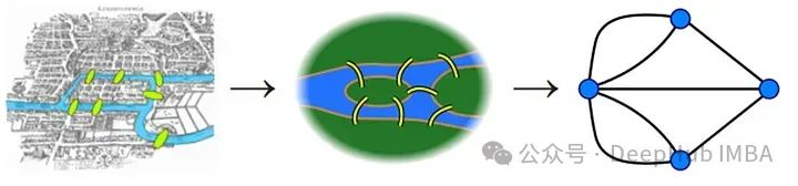
Graph theory was introduced by Euler in the 18th century to solve the famous Königsberg bridge problem: is it possible to cross all seven bridges only once?

What is a Graph? How to Define It?

A graph is a set of interconnected objects.

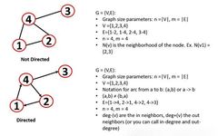
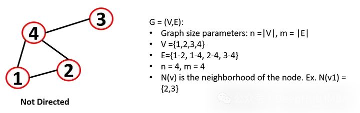
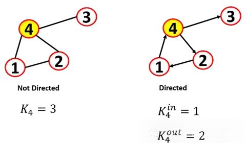
A graph consists of a set of nodes N and edges E, where n is the number of vertices and m is the number of edges. Two connected nodes are defined as adjacent (node 1 is adjacent to node 4). When we refer to the size of the network N, it usually refers to the number of nodes (the number of links or edges is usually referred to as L).

Directed and Undirected

A graph can be either undirected or directed:

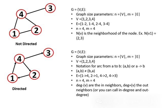
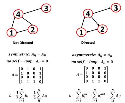
Undirected graph: edges are undirected, and the relationships are symmetric. The order of drawing the edges does not matter.

Directed graph: edges are directed (also known as directed graphs), and the edges between vertices can have a direction, which can be represented with arrows (also known as arcs).

Basic Properties of Graphs

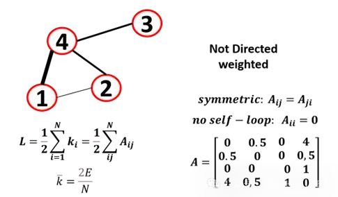
For a node, we can define the node degree (k) as the number of edges adjacent to the node. For a graph, we can calculate the average degree k of an undirected graph:

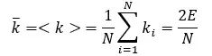
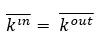
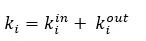
In directed networks, the in-degree (edges pointing to the node) and out-degree (edges leaving the node) of a node are defined, and the total degree of the node is the sum of both. We call a source node a node with no in-degree and a sink node a node with no out-degree.

We can calculate the average degree as follows:

Here,

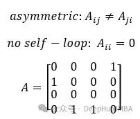
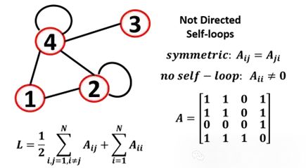
The adjacency matrix is another way to represent a graph, where rows and columns represent graph nodes, and the intersection indicates whether there is a link between two nodes. The size of the adjacency matrix is n x n (number of vertices). If Aij is the link between nodes i and j, then Aij is 1; otherwise, it is 0. For undirected graphs, the matrix is symmetric. The absence of 1 on the diagonal of the matrix indicates no self-loops (nodes connected to themselves).

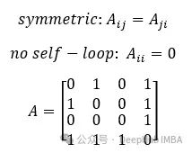
To calculate the number of edges (or its degree) for a node i, sum along the row or column:

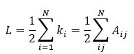
The total number of edges in an undirected graph is the sum of the degrees of each node (which can also be the sum of the values in the adjacency matrix):

Because in undirected graphs, you count the edges twice (due to the adjacency matrix being symmetric), it is divided by 2.

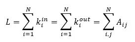
For directed graphs, two different adjacency matrices can be represented, one for in-degree and one for out-degree:

For a node, the total number of edges is the sum of the in-degree and out-degree:

We calculate the in-degree and out-degree of a node as well as the total number of edges:

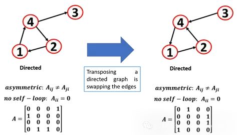
Due to the connection between linear algebra and graph theory, different operations can be applied to the adjacency matrix. If the adjacency matrix of an undirected graph is transposed, the graph remains unchanged because it is symmetric, but if the adjacency matrix of a directed graph is transposed, the direction of the edges is reversed.

These matrices are very sparse because theoretically, a node can connect to all other nodes, but this rarely happens in real life. When all nodes are connected to other nodes, we call it a complete graph. Complete graphs are often used to understand some complex problems in graph theory (e.g., connectivity).

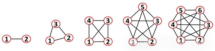
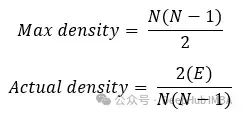
The maximum density of a graph is the total number of possible relationships in a complete graph. The actual density measures the density of undirected non-complete graphs:

Theoretically, in a social network, everyone can connect to everyone, but this does not happen. So ultimately, an adjacency matrix with 7 billion rows and 7 billion columns is obtained, where most entries are zero (because it is very sparse). Why mention this? Because not all algorithms can handle sparse matrices well.

In addition to the adjacency matrix, we can also represent the graph as a list of edges:

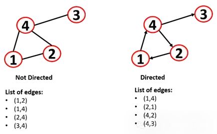
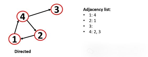
However, this method has issues for machine learning analysis, leading to a commonly used method: adjacency lists, as they are useful for large and sparse nodes, allowing for quick retrieval of a node’s neighbors.

Weighted Graphs

Edges of a graph can also have weights, as not all edges are the same. For example, in a traffic graph, to choose the best path between two nodes, we will consider weights representing time or traffic.

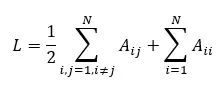
Self-loops

Nodes of a graph can connect to themselves, so self-loops must be added when calculating the total number of edges:

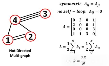
You can also have a multigraph, which has multiple edges between the same pair of nodes:

Multigraphs

A graph containing parallel edges is called a multigraph or has multiple edges between a pair of nodes.

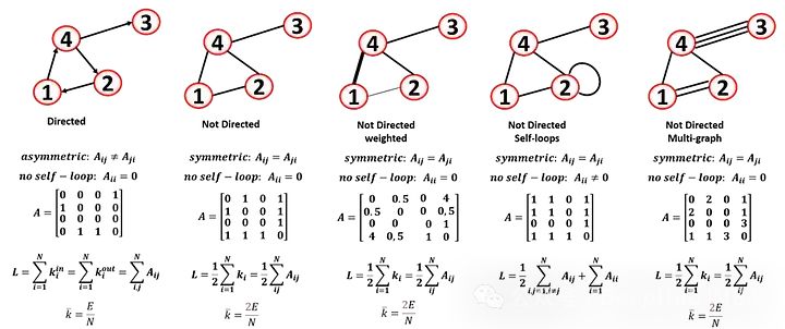
Above are some common graphs and representations; let’s summarize:

Another important parameter of a graph is connectivity. Can every node be reached by all other nodes? A connected graph is one where all vertices can be connected by a path. A disconnected graph is one that has two or more connected components.

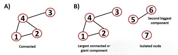
The largest isolated subset of nodes is called an “island.” Knowing whether a graph is connected or disconnected is important, as some algorithms struggle to handle disconnected graphs.

This can be displayed in the adjacency matrix, where different components are written as diagonal blocks (non-zero elements are restricted to square matrices). We call the links that connect two “islands” as “bridges.”

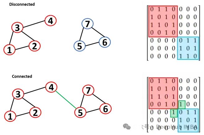
If the graph is small, this visual inspection is easy, but for a large graph, checking connectivity is very challenging.

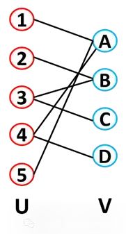
Bipartite Graphs

The graphs we have seen above are called unipartite graphs, which have only one type of node and one type of relationship.

A bipartite graph is a graph that divides nodes into two disjoint sets (usually referred to as U and V). These sets are independent, and every node in set U is connected to some node in set V (each link can only connect a node from one set to a node from the other set). Therefore, a bipartite graph is one that has no U-U connections and no V-V connections. There are many such examples: authors to papers (authors in set U connected to papers in set V), actors (U) and the movies they starred in (V), users and products, recipes and ingredients, etc. Another example is disease networks, which include a set of diseases and a set of genes, where only genes with known mutations that cause or affect the disease are connected to the disease. Another example is matching, where bipartite graphs can be used in dating applications. For a bipartite graph with two sets of nodes (U has m nodes, V has n nodes), the total number of possible edges is m*n, and the total number of nodes is m + n.

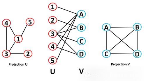
Bipartite graphs can be folded into two separate networks, the projection of U and the projection of V. In the projection of U, if two nodes are connected to the same V node, they are connected (the principle is the same for the V projection).

If needed, we can also construct a tripartite graph. Overall, you can have more than three types of nodes; we usually talk about k-partite graphs. This type of graph extends our view of bipartite graphs.

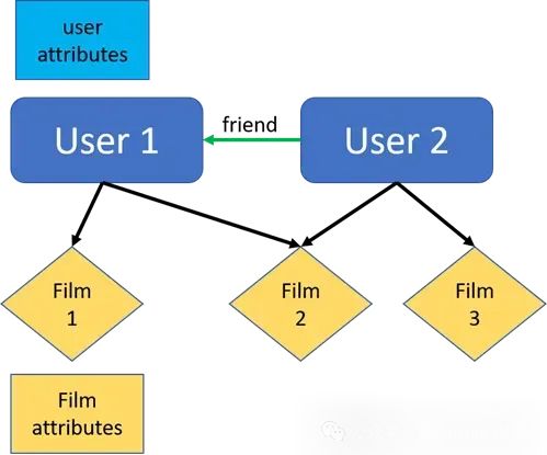
Heterogeneous Graphs

A heterogeneous graph (also known as a heterogeneous graph) is a graph that has different types of nodes and edges.

Planar Graphs

A graph that can be drawn in a form without any edges intersecting (for a graph, if it can be drawn in this way, it is called a planar representation) can be considered a planar graph. Even if the edges intersect when drawn, the graph can still be planar. Look at this example; this graph can be redrawn as a planar representation.

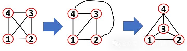
Why is it useful to know whether we can have a planar representation? One of the most common examples is drawing circuit boards to ensure that the circuits do not intersect.

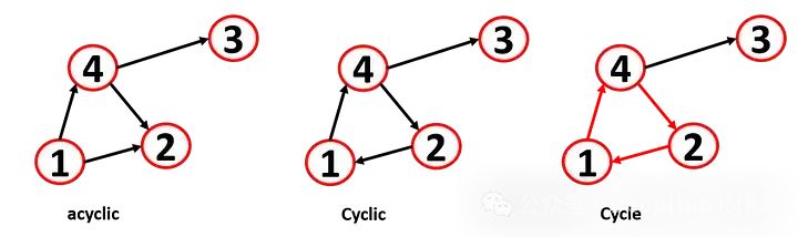
Cyclic and Acyclic Graphs

A walk is an alternating sequence of nodes (a walk from u to v is a sequence of nodes starting at u and ending at v). A path is a walk where all nodes in the sequence are distinct (u-x-v is a path, but u-x-u-x-v is a walk but not a path). A cyclic graph is one where the path starts and ends at the same node, as different algorithms have cycle issues (sometimes requiring converting cyclic graphs to acyclic graphs by cutting some connections). We can define feedforward neural networks as directed acyclic graphs (DAGs) because DAGs always have an endpoint (also known as a leaf node).

Conclusion

In this article, we introduced what a graph is and its main attributes. Although graphs may seem simple, they can realize infinite variations. A graph is a collection of nodes and edges; it has no order, no start, and no end. We can define different types of concepts and data through them. Graphs can also succinctly describe many properties of data and provide us with information about the relationships between different subjects. For example, we can assign weights and attributes to nodes and edges. In later articles, we will discuss how to use algorithms in these networks (and how to represent them).