Core Points:A comprehensive summary of machine learning concepts, highly recommended for collection!

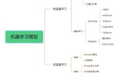
1. Supervised Learning
Supervised learning typically uses training data with expert-labeled tags to learn a function mapping from input variable X to output variable Y. Y = f(X), where the training data is usually in the form of (n×x, y), with n representing the size of the training sample, and x and y being the sample values of variables X and Y, respectively.
Supervised learning can be divided into two categories:
-
Classification problems: predicting the category of a sample (discrete). For example, determining gender, health status, etc.
-
Regression problems: predicting the corresponding real number output of a sample (continuous). For example, predicting the average height of people in a certain area.
Additionally, ensemble learning is also a type of supervised learning. It combines the predictions of multiple relatively weak machine learning models to predict new samples.
1.1 Single Models
1.11 Linear Regression
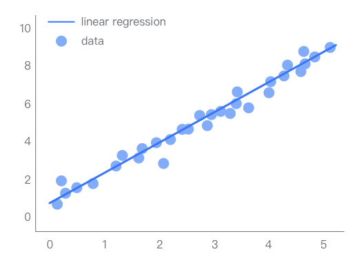
Linear regression refers to a regression model composed entirely of linear variables. In linear regression analysis, there is only one independent variable and one dependent variable, and their relationship can be approximated by a straight line. This type of regression analysis is called univariate linear regression analysis. If the regression analysis includes two or more independent variables, and the relationship between the dependent variable and the independent variables is linear, it is called multivariate linear regression analysis.
1.12 Logistic Regression
This is used to study the influence relationship between X and Y when Y is categorical data. If Y has two categories, such as 0 and 1 (where 1 means willing and 0 means not willing, 1 means purchase and 0 means no purchase), it is called binary logistic regression; if Y has three or more categories, it is called multiclass logistic regression.
The independent variable does not necessarily have to be categorical; they can also be quantitative variables. If X is categorical data, dummy variable settings are required for X.
1.13 Lasso
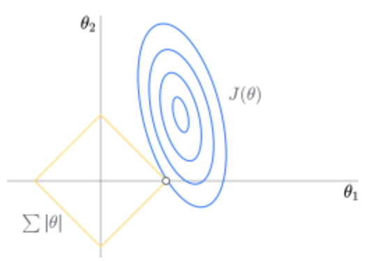
The Lasso method is a compressed estimation method that serves as an alternative to the least squares method. The basic idea of Lasso is to establish an L1 regularization model, which compresses some coefficients and sets some coefficients to zero during the model establishment process. After the model training is complete, parameters with weights equal to 0 can be discarded, making the model simpler and effectively preventing overfitting. It is widely used for fitting and variable selection in the presence of multicollinearity data.
1.14 K-Nearest Neighbors (KNN)
The main difference between KNN for regression and classification lies in the decision-making method during prediction. For classification predictions, KNN generally uses majority voting, meaning it predicts the class with the most occurrences among the K nearest samples in the training set. For regression, it typically uses the average of the outputs from the K nearest samples as the regression prediction value. However, their theories are the same.
1.15 Decision Trees
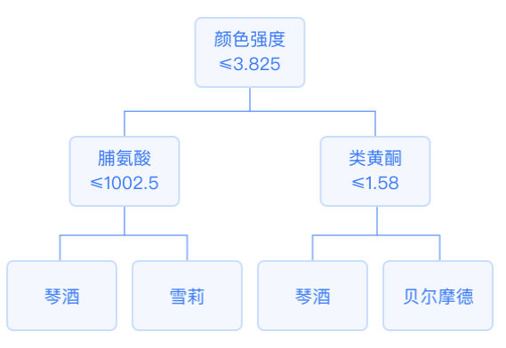
In a decision tree, each internal node represents a splitting problem: it specifies a test on a certain attribute of instances, dividing the samples arriving at that node based on a specific attribute, with each successor branch corresponding to a possible value of that attribute. The output variable’s mode in the leaf nodes of a classification tree is the classification result. The output variable’s mean in the leaf nodes of a regression tree is the prediction result.
1.16 BP Neural Networks
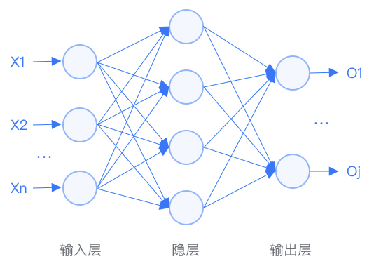
BP neural networks are a type of multilayer feedforward network trained by the error backpropagation algorithm, and they are one of the most widely used neural network models today. The learning rule of BP neural networks uses the steepest descent method to continuously adjust the network’s weights and thresholds through backpropagation, minimizing the classification error rate (minimizing the sum of squared errors).
The BP neural network is a multilayer feedforward neural network characterized by forward propagation of signals and backward propagation of errors. Specifically, for a neural network model containing only one hidden layer:
The process of the BP neural network is mainly divided into two stages. The first stage is the forward propagation of signals from the input layer through the hidden layer to the output layer. The second stage is the backward propagation of errors from the output layer to the hidden layer, finally to the input layer, adjusting the weights and biases from the hidden layer to the output layer, and from the input layer to the hidden layer.
1.17 Support Vector Machines (SVM)
Support Vector Regression (SVR) uses nonlinear mapping to map data into a high-dimensional feature space, allowing independent and dependent variables to exhibit good linear regression characteristics in that space, fitting in that feature space and then returning to the original space.
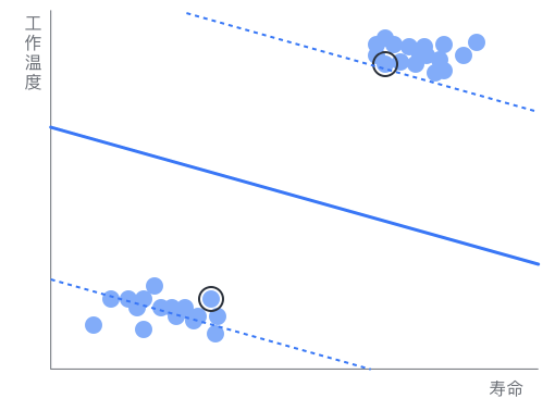
Support Vector Classification (SVM) is a type of generalized linear classifier that performs binary classification on data using supervised learning, with its decision boundary being the maximum margin hyperplane obtained from the learning samples.
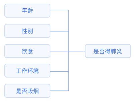
1.18 Naive Bayes
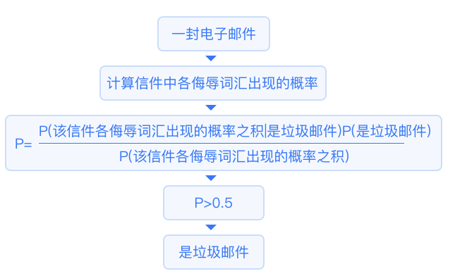
Given the premise of one event occurring, we calculate the probability of another event occurring using Bayes’ theorem. Assuming prior knowledge is d, to calculate the probability of our hypothesis h being true, we will use the following Bayes’ theorem:
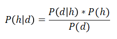
This algorithm assumes that all variables are independent of each other.
1.2 Ensemble Learning
Ensemble learning is a method that combines the results of different learning models (such as classifiers) to further improve accuracy through voting or averaging. Generally, voting is used for classification problems, and averaging is used for regression problems. This practice is based on the idea that “many hands make light work”.
Ensemble algorithms can be divided into three main categories: Bagging, Boosting, and Stacking. This article will not discuss stacking.

-
Boosting

1.21 GBDT
GBDT is a Boosting algorithm with CART regression trees as the base learner. It is an additive model that sequentially trains a set of CART regression trees, ultimately summing the predictions of all regression trees to obtain a strong learner. Each new tree fits the negative gradient direction of the current loss function. Finally, the sum of this set of regression trees outputs the regression result or applies the sigmoid or softmax function to obtain binary or multiclass results.
1.22 AdaBoost
AdaBoost assigns a high weight to learners with low error rates and a low weight to learners with high error rates, combining weak learners with their corresponding weights to generate a strong learner. The difference between regression and classification algorithms lies in how error rates are calculated; classification problems generally use a 0/1 loss function, while regression problems typically use squared loss functions or linear loss functions.
1.23 XGBoost
XGBoost stands for “Extreme Gradient Boosting,” which is a class of composite algorithms that combine base functions and weights to fit data effectively. Due to its strong generalization ability, high scalability, and fast computation speed, XGBoost has been well-received in statistics, data mining, and machine learning since its introduction in 2015.
XGBoost is an efficient implementation of GBDT, and unlike GBDT, it adds a regularization term to the loss function; since some loss functions are difficult to compute derivatives for, XGBoost uses the second-order Taylor expansion of the loss function for fitting.
1.24 LightGBM
LightGBM is an efficient implementation of XGBoost, which discretizes continuous floating-point features into k discrete values and constructs a histogram with a width of k. It then traverses the training data to calculate cumulative statistics for each discrete value in the histogram. When performing feature selection, it only needs to find the optimal split points based on the discrete values in the histogram, using a leaf-wise growth strategy with depth restrictions to save time and space costs.
1.25 CatBoost
CatBoost is a GBDT framework based on symmetric decision trees, primarily designed to efficiently and reasonably handle categorical features, as well as address gradient bias and prediction shift issues, improving the algorithm’s accuracy and generalization ability.
-
Bagging
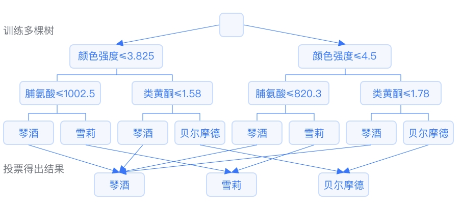
1.26 Random Forest
Random forest classification generates numerous decision trees by randomly sampling both the observed samples and feature variables from the modeling dataset. Each sampling result corresponds to a tree, and each tree generates rules and classification results (judgment values) that conform to its own attributes. The forest ultimately integrates all decision trees’ rules and classification results (judgment values) to implement the random forest algorithm’s classification (regression).
1.27 Extra Trees
Extra Trees (Extremely Randomized Trees) are very similar to random forests, with the term “extremely random” reflecting the random feature and threshold divisions used in decision trees. This means that each decision tree’s shape and differences will be greater and more random.
2. Unsupervised Learning
Unsupervised learning problems deal with training data that only contains input variable X without corresponding output variables. It models the structure of the data without expert-labeled training data.
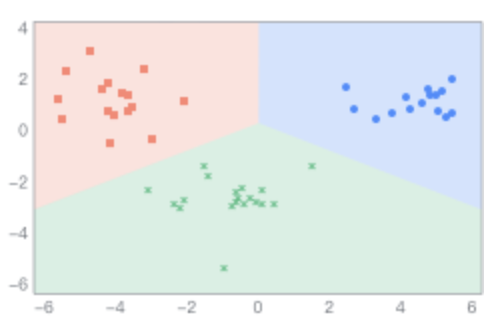
2.1 Clustering
Clustering divides similar samples into a cluster. Unlike classification problems, clustering problems do not know the categories in advance, and naturally, the training data lacks category labels.
2.11 K-means Algorithm
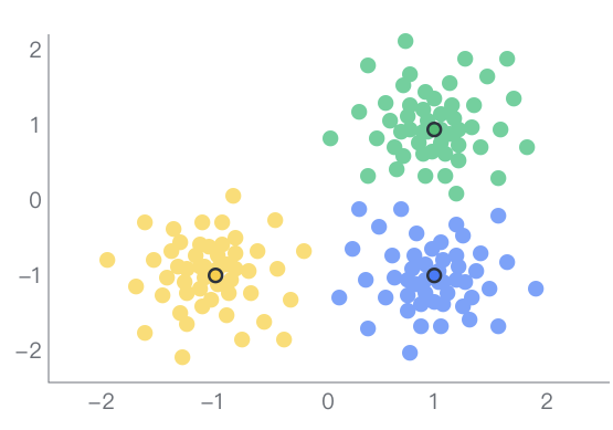
Clustering analysis is a center-based clustering algorithm (K-means clustering) that iteratively assigns samples to K classes, minimizing the sum of distances between each sample and the center or mean of its assigned class. Unlike hierarchical clustering algorithms that cluster based on fields, fast clustering analysis clusters based on samples.
2.12 Hierarchical Clustering
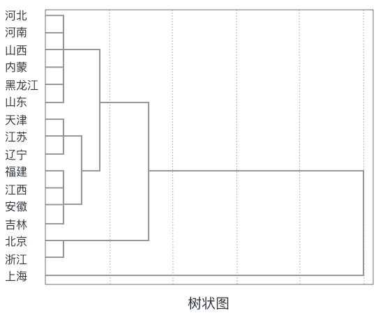
Hierarchical clustering is a type of clustering that performs hierarchical decomposition of a given set of data objects based on a chosen decomposition strategy. Hierarchical clustering algorithms build clusters hierarchically, forming a tree with clusters as nodes. If the decomposition is performed from the bottom up, it is called agglomerative hierarchical clustering, such as AGNES. If it is performed from the top down, it is called divisive hierarchical clustering, such as DIANA. Generally, agglomerative hierarchical clustering is more commonly used.
2.2 Dimensionality Reduction
Dimensionality reduction refers to reducing the dimensions of data while preserving meaningful information. This can be achieved through feature extraction and feature selection methods. Feature selection refers to selecting a subset of the original variables, while feature extraction transforms data from high dimensions to low dimensions. A widely known method for feature extraction is Principal Component Analysis (PCA).
2.21 PCA (Principal Component Analysis)
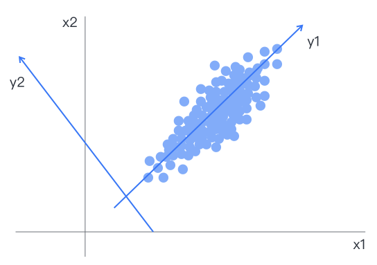
PCA combines multiple correlated indicators linearly to explain as much information as possible from the original data with the least dimensions. The variables after dimensionality reduction are linearly independent of each other, and the newly determined variables are linear combinations of the original variables, with the proportion of variance explained by later principal components decreasing.
2.22 SVD (Singular Value Decomposition)
SVD is a widely used algorithm in machine learning, applicable not only in dimensionality reduction algorithms for eigenvalue decomposition but also in recommendation systems and natural language processing, serving as the foundation for many algorithms.
2.23 LDA (Linear Discriminant Analysis)
The principle of linear discriminant is to project samples onto a line in such a way that the projection points of the same class are as close as possible, while the projection points of different classes are as far apart as possible. When classifying new samples, they are projected onto the same line, and their class is determined based on the position of the projection point.
In Conclusion
This article is from SPSSPRO, providing a comprehensive summary of machine learning concepts. It is highly recommended to collect and read it slowly. The full text elaborates on various details of algorithms in both supervised and unsupervised learning!
If you like it, feel free to collect, like, and share it!