
Source: DeepHub IMBA


This article is approximately 4600 words long and is recommended to be read in 10 minutes.
In this article, we will combine text and knowledge graphs to enhance the performance of our RAG.
In our previous articles, we introduced examples of combining knowledge graphs with RAG. In this article, we will combine text and knowledge graphs to enhance the performance of our RAG.
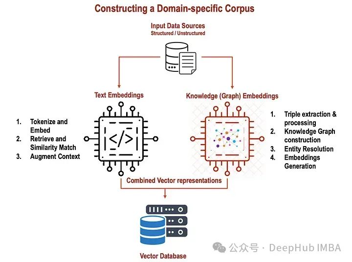
Text Embeddings in RAG
Text embeddings are numerical representations of words or phrases that can effectively capture their meanings and contexts. They can be viewed as unique identifiers for words—a concise vector that encapsulates the meanings of the words they represent. These embeddings enable computers to enhance their understanding and processing of text, allowing them to excel in various NLP tasks such as text classification, sentiment analysis, and machine translation.
Pre-trained models such as Word2Vec, GloVe, or BERT can be utilized to generate text embeddings. These models have been extensively trained on large amounts of text data and have acquired the ability to encode semantic information about words and their relationships.
Let’s explore the process of generating text embeddings using a simple Python code snippet (word2vec):
# Code Implementation: Generating Text Embeddings
import numpy as np
from gensim.models import Word2Vec

# Sample sentences
sentences = [
    ["I", "love", "natural", "language", "processing"],
    ["Text", "embeddings", "are", "fascinating"],
    ["NLP", "makes", "computers", "understand", "language"]
]

# Train Word2Vec model
model = Word2Vec(sentences, vector_size=5, window=5, min_count=1, sg=1)

# Get embeddings for words
word_embeddings = {}
for word in model.wv.index_to_key:
    word_embeddings[word] = model.wv[word]

# Print embeddings for word, embedding in word_embeddings.items():
    print(f"Embedding for '{word}': {embedding}")
In this code snippet, we develop a Word2Vec model by training it on a set of sample sentences. The model then generates embeddings for each word. These embeddings capture the semantic relationships between words in the sentences. The code snippet for generating text embeddings using Word2Vec outputs the following:
Embedding for 'I': [-0.01978252 0.02348454 -0.0405227 -0.01806103 0.00496107]
Embedding for 'love': [ 0.01147135 -0.00716509 -0.02319919 0.03274594 -0.00713439]
Embedding for 'natural': [ 0.03319094 0.02570618 0.02645341 -0.00284445 -0.01343429]
Embedding for 'language': [-0.01165106 -0.02851446 -0.01676577 -0.01542572 -0.02357706]

In the output above:
Each line corresponds to an embedding vector for a word. Each line starts with the word followed by the embedding vector represented as a list of values. For example, the embedding for the word “love” is: [-0.01978252 0.02348454 -0.0405227 -0.01806103 0.00496107].
RAGs utilize text embeddings to grasp the context of input queries and extract relevant information.
Now let’s attempt to tokenize and encode the input query using a pre-trained model (such as BERT). This will convert the query into a numerical representation that captures its semantics and context.
# Code Implementation: Tokenization and Encoding
from transformers import BertTokenizer, BertModel

# Initialize BERT tokenizer and model
tokenizer = BertTokenizer.from_pretrained('bert-base-uncased')
model = BertModel.from_pretrained('bert-base-uncased')

# Tokenize and encode the input query
query = "What is the capital of France?"
input_ids = tokenizer.encode(query, add_special_tokens=True, return_tensors="pt")
We use BERT to tokenize the input query and encode it into numerical IDs. Since the initialization and tokenization process of the BERT model involves loading a large pre-trained model, the output of the tokenization and encoding steps includes the following components:
ID: These are the numerical representations of the tokens in the input query. Each token is converted into an ID that corresponds to an index in the BERT vocabulary.
Attention Mask: This is a binary mask indicating which tokens are actual words (1) and which are padding tokens (0). It ensures that the model only focuses on real tokens during processing.
Token Type ID (for models like BERT): In cases of multiple segments, it indicates which segment or sentence each token belongs to. For single-sentence inputs, all token type IDs are usually set to 0.
The output is a dictionary containing these components, which can be used as input to the BERT model for further processing.
Below is an example of the output:
{
    'input_ids': tensor([[ 101, 2054, 2003, 1996, 3007, 1997, 2605, 1029,   102,     0]]),
    'attention_mask': tensor([[1, 1, 1, 1, 1, 1, 1, 1, 1, 0]]),
    'token_type_ids': tensor([[0, 0, 0, 0, 0, 0, 0, 0, 0, 0]])
}

input_ids contain the numerical IDs of the tokens in the input query. Attention_mask indicates which tokens are actual words (1) and which are padding tokens (0). Token_type_ids indicate the segment or sentence each token belongs to (in this case, the first sentence is 0).
Next, relevant paragraphs can be retrieved from the corpus based on the encoded query. We use cosine similarity to compute the similarity score between the query embedding and the paragraph embeddings.
# Code Implementation: Retrieval and Similarity Matching
from sklearn.metrics.pairwise import cosine_similarity

# Retrieve passages and compute similarity scores
query_embedding = model(input_ids)[0].mean(dim=1).detach().numpy()
passage_embeddings = ... # Retrieve passage embeddings
similarity_scores = cosine_similarity(query_embedding, passage_embeddings)
Select the passage with the highest similarity score and output it along with its similarity score. The similarity score indicates how similar each paragraph is to the input query, with higher scores indicating greater similarity. In the RAG model, the article with the highest similarity score is considered the most relevant for further processing.
Finally, we designate the passage with the highest similarity score as the most relevant article. This segment provides relevant information for the generation phase of the model.
# Select passage with highest similarity score
max_similarity_index = np.argmax(similarity_scores)
selected_passage = passages[max_similarity_index]

# Output selected passage and similarity score
print("Selected Passage:")
print(selected_passage)
print("Similarity Score:", similarity_scores[0][max_similarity_index])
Text embeddings are a very powerful tool in the field of natural language processing (NLP) that can effectively understand and process textual information. They have significant impacts on many tasks, such as question answering, text generation, and sentiment analysis. By using text embeddings in RAG, performance and accuracy can be improved, leading to more accurate and contextually relevant responses.
Knowledge Graph Embeddings in RAG
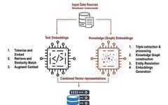
Next, we will introduce how to define and implement knowledge graph embeddings to represent structured domains from unstructured data.
A knowledge graph is a very effective way to organize information and connect entities and their relationships in a meaningful way. These graphs act like a well-organized information warehouse, capturing the meanings of objects in the real world and their connections. However, this process does not end with the development of the knowledge graph. Exploring the field of knowledge graph embeddings is crucial to unlocking its full potential.
To demonstrate, we maintain the basic structure of the KG but simplify the use of KG components. After representing KG elements as embeddings, a scoring function is used to evaluate the plausibility of triples, such as “Tim”, “is an”, “Artist”.
Here are the steps to implement knowledge (graph) embeddings:
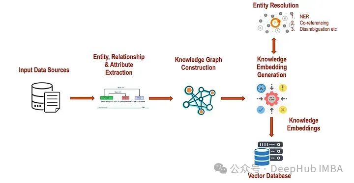
Given an unstructured text, we will first extract key entities, relationships, and attributes using Stanford’s OpenIE framework. Once the triples are extracted, we can clean/adjust them.
from openie import StanfordOpenIE
text = "Hawaii is a state in the United States. Barack Obama served as the 44th president of the United States. The Louvre Museum is located in Paris, France."

with StanfordOpenIE() as client:
    triples = client.annotate(text)
    for triple in triples:
        print(triple)
    cleaned_triples = [(subject.lower(), relation.lower(), object.lower()) for (subject, relation, object) in triples]
    print("Cleaned Triples:", cleaned_triples)
The output of the code above is:
('Hawaii', 'is', 'a state in the United States')
('Barack Obama', 'served as', 'the 44th president of the United States')
('The Louvre Museum', 'is located in', 'Paris, France')
Cleaned Triples: [('hawaii', 'is', 'a state in the united states'), ('barack obama', 'served as', 'the 44th president of the united states'), ('the louvre museum', 'is located in', 'paris, france')]
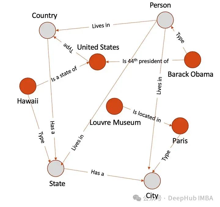
Now we can use this information to create a knowledge graph, constructing a graph with entities as nodes and relationships as edges using the NetworkX framework. Here is the implementation:
import networkx as nx

# Create a directed graph
knowledge_graph = nx.DiGraph()

# Add nodes and edges from cleaned triples
for (subject, relation, object) in cleaned_triples:
    knowledge_graph.add_edge(subject, object, relation=relation)

# Visualize the knowledge graph
nx.draw(knowledge_graph, with_labels=True)
Entity resolution plays a critical role in various NLP applications, including information extraction, question answering, and knowledge graph construction. By accurately linking mentions of entities in text to corresponding entities in structured knowledge representations, entity resolution enables machines to utilize natural language understanding and reasoning more effectively, facilitating a wide range of downstream tasks and applications.
Entity resolution addresses the challenges of ambiguity and variability in natural language. In everyday language use, different names, synonyms, abbreviations, or variants are often used to refer to entities such as people, places, organizations, and concepts. For instance, “Barack Obama” may be referred to as “Obama,” “former president of the United States,” or simply “he.” There may also be entities with similar names or attributes, leading to potential confusion or ambiguity. For example, “Paris” can refer to the capital of France or other places with the same name.
We briefly introduce each type of entity resolution technique:
Exact Matching: In the text, mentioning “Hawaii” can be directly linked to the node marked as “Hawaii” in the graph because they match exactly.
Partial Matching: If the text mentions “USA” instead of “United States,” a partial matching algorithm might recognize the similarity between the two and link the mention to the node marked as “United States” in the graph.
Named Entity Recognition (NER): Using NER, the system can identify “Barack Obama” as a personal entity mentioned in the text. This mention can then be linked to the corresponding node marked as “Barack Obama” in the graph.
Coreference Resolution: If the text mentions “he served as president,” coreference resolution can link “he” back to “Barack Obama” mentioned earlier in the text, and then link it to the node marked as “Barack Obama” in the graph.
Disambiguation: Suppose the text mentions “Paris” without specifying whether it refers to the city in France or another place. Disambiguation techniques may consider contextual information or external knowledge sources to determine that it refers to “Paris, France,” and link it to the corresponding node in the graph.
Once the correct entity links are determined, mentions in the text will be linked to the corresponding entities in the knowledge base or knowledge graph. The performance of entity resolution systems is evaluated using metrics such as precision, recall, and F1 score, comparing predicted entity links with ground truth or standards. Below is an example of entity resolution on the constructed graph above. The gray circles represent the class types of the given entities.
As a final step, we will now generate embeddings for entities and relationships. We will use TransE here.
from pykeen.pipeline import pipeline

# Define pipeline configuration
pipeline_config = {
    "dataset": "nations",
    "model": {
        "name": "TransE",
        "embedding_dim": 50
    },
    "training": {
        "num_epochs": 100,
        "learning_rate": 0.01
    }
}

# Create and run pipeline
result = pipeline(
    **pipeline_config,
    random_seed=1234,
    use_testing_data=True
)

# Access trained embeddings
entity_embeddings = result.model.entity_embeddings
relation_embeddings = result.model.relation_embeddings

# Print embeddings
print("Entity Embeddings:", entity_embeddings)
print("Relation Embeddings:", relation_embeddings)
The output obtained is as follows:
Entity Embeddings: [Embedding dimension: (120, 50)]
Relation Embeddings: [Embedding dimension: (120, 50)]
Integrating Text and Knowledge Graphs
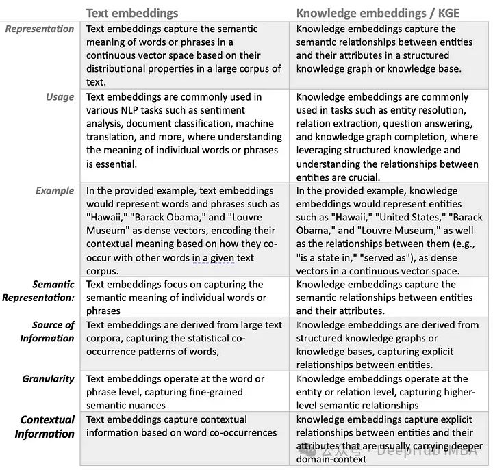
Before we combine these embeddings, we must first understand their objectives and verify that they are fully complementary.
Text embeddings and knowledge graph embeddings serve different purposes in natural language processing (NLP), representing different aspects of language and semantic information.
The following code integrates text embeddings and knowledge embeddings into a single embedding space, and then retrieves relevant paragraphs from the knowledge base based on the cosine similarity between the combined embeddings of the query and paragraphs. The output shows the relevant paragraphs along with their similarity scores to the query.
import numpy as np
from sklearn.metrics.pairwise import cosine_similarity

# Sample knowledge embeddings
knowledge_embeddings = { } #initialize the above knowledge embeddings output

# Sample text embeddings
text_embeddings = { } #initialize the above text embeddings output

# Consider passages from knowledge base
knowledge_base = {
    "Passage 1": "Hawaii is a state in the United States.",
    "Passage 2": "Barack Obama served as the 44th president of the United States.",
    # Add more passages as needed
}

# Function to combine text and knowledge embeddings
def combine_embeddings(text_emb, know_emb):
    combined_emb = {}
    for entity, t_emb in text_emb.items():
        if entity in know_emb:
            combined_emb[entity] = np.concatenate([t_emb, know_emb[entity]])
        else:
            combined_emb[entity] = t_emb
    return combined_emb

# Function to retrieve relevant passages using combined embeddings
def retrieve_passages(query_emb, knowledge_base_emb):
    similarities = {}
    for passage, kb_emb in knowledge_base_emb.items():
        sim = cosine_similarity([query_emb], [kb_emb])[0][0]
        similarities[passage] = sim
    sorted_passages = sorted(similarities.items(), key=lambda x: x[1], reverse=True)
    return sorted_passages

# Example usage
combined_embeddings = combine_embeddings(text_embeddings, knowledge_embeddings)
query = "query"
relevant_passages = retrieve_passages(combined_embeddings[query], knowledge_embeddings)

# Print relevant passages
for passage, similarity in relevant_passages:
    print("Passage:", passage)
    print("Similarity:", similarity)
The output is as follows:
Passage: Passage 1 Similarity: 0.946943628930774
Passage: Passage 2 Similarity: 0.9397945401928656
Conclusion
Using both text embeddings and knowledge embeddings in RAG can enhance the model’s performance and capabilities in several ways:
1. Text embeddings capture the semantics of individual words or phrases, while knowledge embeddings capture explicit relationships between entities. By integrating both types of embeddings, the RAG model achieves a more comprehensive grasp of the input text and the organized information stored in the knowledge graph.
2. Text embeddings provide valuable contextual insights by analyzing word co-occurrences in the input text, while knowledge embeddings provide contextual relevance by examining the relationships between entities in the knowledge graph. By combining different types of embeddings, the RAG model can generate responses that are semantically relevant to the input text and contextually consistent with structured knowledge.
3. The integration of knowledge embeddings in the retrieval component significantly enhances answer selection in the RAG model. By indexing and retrieving relevant paragraphs in the knowledge base using knowledge embeddings, the RAG model can not only retrieve more accurate responses but also provide richer information.
4. Text embeddings enhance the generative component of the RAG model by incorporating a wide range of linguistic features and semantic nuances. By integrating text embeddings and knowledge embeddings in the answer generation process, the RAG model can generate responses that are linguistically fluent, semantically relevant, and grounded in structured knowledge.
5. By using text embeddings and knowledge embeddings, the RAG model gains enhanced resilience to ambiguity and variability in natural language. Text embeddings capture the variability and ambiguity present in unstructured text, while knowledge embeddings provide explicit semantic relationships that enhance and clarify the model’s understanding.
6. Knowledge embeddings allow the RAG model to seamlessly integrate structured knowledge from the knowledge base into the generation process. Through the integration of knowledge embeddings and text embeddings, the RAG model achieves a seamless fusion of structured knowledge and unstructured text, resulting in richer information and contextually relevant responses.
In the RAG model, both text embeddings and knowledge embeddings enable a more comprehensive and context-rich representation of input text and structured knowledge. This integration enhances the model’s performance in answer retrieval, answer generation, robustness to ambiguity, and effective integration of structured knowledge, ultimately leading to more accurate and informative responses.
Editor: Huang Jiyan