Source: CSDN Blog
Author: Jay Alammar
This article is about 7293 words, suggested reading time 14 minutes。
This article introduces knowledge related to the Transformer, using a simplified model to explain core concepts one by one.
The Transformer was proposed in the paper “Attention is All You Need” and is now recommended as a reference model by Google Cloud TPU. The Tensorflow code related to the paper can be obtained from GitHub as part of the Tensor2Tensor package. Harvard’s NLP team has also implemented a version based on PyTorch and annotated the paper.
In this article, we will try to simplify the model a bit and introduce the core concepts one by one, hoping to make it easy for the average reader to understand.
Attention is All You Need:
https://arxiv.org/abs/1706.03762
Starting from a macro perspective:
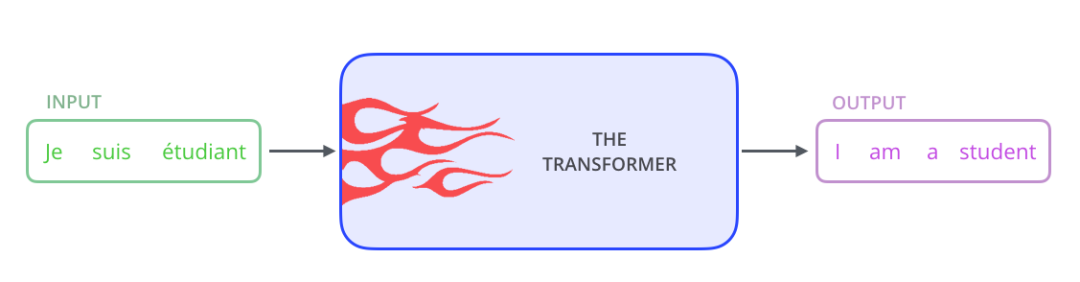
First, consider this model as a black box operation. In machine translation, it is inputting one language and outputting another language.
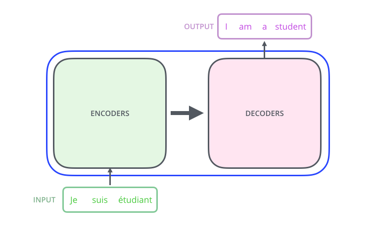
By breaking open this black box, we can see that it consists of an encoding component, a decoding component, and the connections between them.
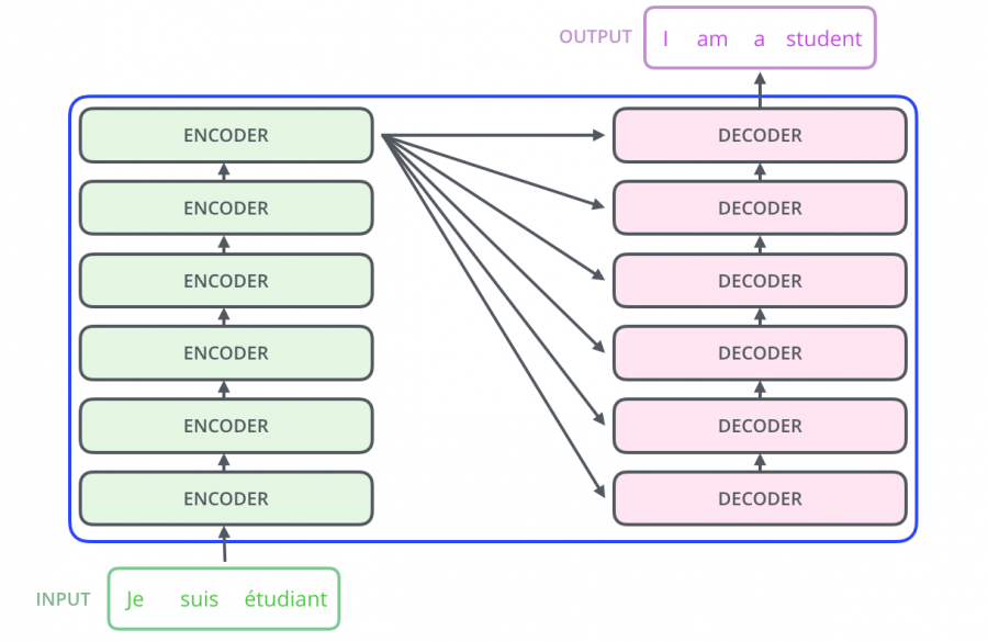
The encoding component is composed of a stack of encoders (the paper stacks six encoders together – the number six is not magical, you can try other numbers).
The decoding component also consists of the same number (corresponding to the encoders) of decoders.
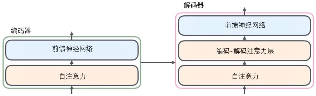
All encoders are structurally the same, but they do not share parameters. Each decoder can be decomposed into two sub-layers.
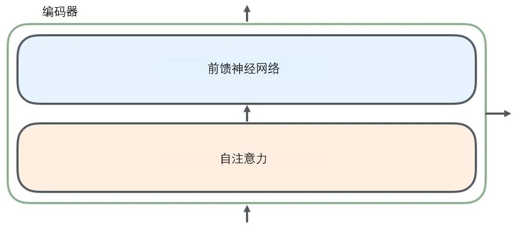
The sentence input from the encoder first goes through a self-attention layer, which helps the encoder focus on other words in the input sentence while encoding each word. We will delve deeper into self-attention in a later article.
The output of the self-attention layer is passed to a feed-forward neural network. The feed-forward neural network corresponding to each position’s word is identical (another interpretation is that it is a one-dimensional convolutional neural network with a window size of one word).
The decoder also has self-attention layers and feed-forward layers from the encoder. In addition, there is an attention layer between these two layers to focus on relevant parts of the input sentence (similar to the attention function in seq2seq models).
Introducing Tensors into the Picture:
We have understood the main parts of the model, next, we will look at how various vectors or tensors (the concept of tensors is an extension of the concept of vectors, where we can simply understand a vector as a first-order tensor and a matrix as a second-order tensor) transform the input into output in different parts of the model.
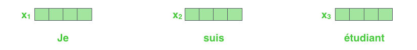
Like most NLP applications, we first convert each input word into a word vector using a word embedding algorithm.
Each word is embedded as a 512-dimensional vector, and we represent these vectors with simple boxes.
The word embedding process occurs only in the bottom-level encoder. All encoders have the same characteristic, which is that they receive a list of vectors, with each vector being 512-dimensional. In the bottom-level (first) encoder, it is the word vector, but in other encoders, it is the output of the next layer encoder (which is also a list of vectors). The size of the vector list is a hyperparameter we can set – generally the length of the longest sentence in our training set.
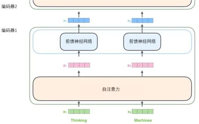
After embedding the input sequence, each word will pass through the two sub-layers in the encoder.
Next, let’s take a look at one of the core features of the Transformer, where each word in the input sequence has its unique path flowing into the encoder. In the self-attention layer, there are dependencies between these paths. However, the feed-forward layer does not have these dependencies. Therefore, various paths can be executed in parallel during the feed-forward layer.
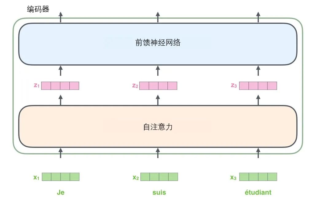
Then we will take a shorter sentence as an example to see what happens in each sub-layer of the encoder.
As mentioned above, an encoder receives a list of vectors as input, then passes the vectors in the list to the self-attention layer for processing, and then passes the results to the feed-forward neural network layer, which passes the output to the next encoder.
Each word in the input sequence undergoes a self-encoding process. Then, they each pass through the same feed-forward neural network – the same network, and each vector goes through it respectively.
Macro Perspective on Self-Attention Mechanism:
Don’t be confused by my use of the term self-attention as if everyone should be familiar with this concept. In fact, I didn’t understand this concept until I read the paper “Attention is All You Need”. Let’s refine how it works.
For example, the following sentence is the input sentence we want to translate:
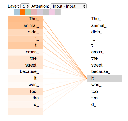
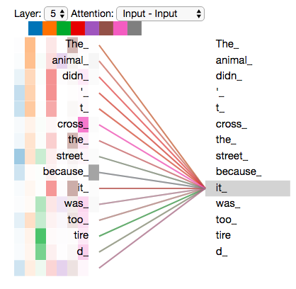
The animal didn’t cross the street because it was too tired
What does this “it” refer to in this sentence? Does it refer to the street or the animal? This is a simple question for humans, but not for algorithms.
When the model processes the word “it”, the self-attention mechanism allows “it” to connect with “animal”.
As the model processes each word in the input sequence, self-attention focuses on all words in the entire input sequence, helping the model to better encode the current word.
If you are familiar with RNNs (Recurrent Neural Networks), recall how it maintains the hidden layer. RNNs combine the representations of all previously processed words/vectors with the current word/vector they are processing. The self-attention mechanism incorporates the understanding of all relevant words into the word we are processing.
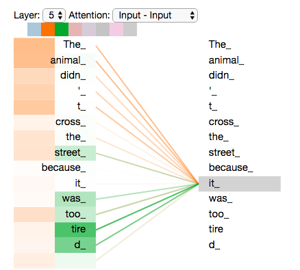
When we encode the word “it” in encoder #5 (the top encoder in the stack), the attention mechanism focuses on “The Animal”, incorporating part of its representation into the encoding of “it”.
Please be sure to check the Tensor2Tensor notebook, where you can download a Transformer model and verify it interactively.
Micro Perspective on Self-Attention Mechanism:
First, let’s understand how to use vectors to calculate self-attention, and then see how it is implemented using matrices.
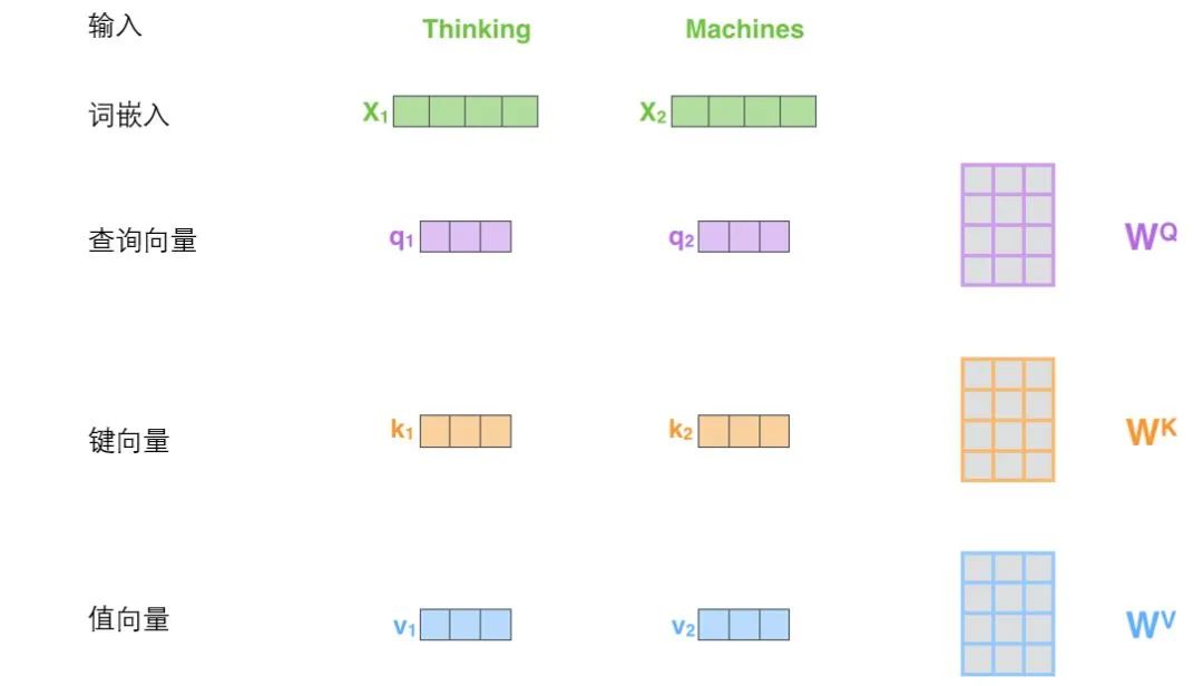
The first step in calculating self-attention is to generate three vectors from each encoder’s input vector (the word vector for each word). That is, for each word, we create a query vector, a key vector, and a value vector. These three vectors are created by multiplying the word embedding with three weight matrices.
It can be observed that these new vectors have a lower dimension than the word embedding vectors. Their dimensions are 64, while the dimensions of the word embedding and encoder input/output vectors are 512. However, it is not strictly required to have a smaller dimension; this is just an architectural choice that allows most of the calculations of multi-headed attention to remain unchanged.
X1 multiplied by the WQ weight matrix gives q1, which is the query vector related to this word. Ultimately, each word in the input sequence creates a query vector, a key vector, and a value vector.
What are query vectors, key vectors, and value vectors?
They are all abstract concepts that help in calculating and understanding the attention mechanism. Please continue reading the content below, and you will know what role each vector plays in calculating the attention mechanism.
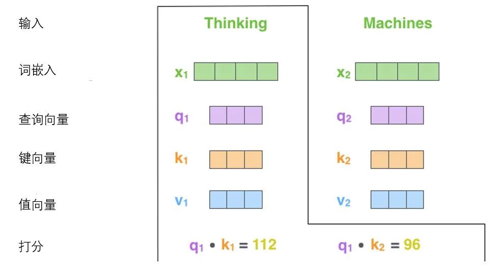
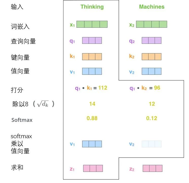
The second step in calculating self-attention is to compute the scores. Suppose we are calculating the self-attention vector for the first word “Thinking” in this example, we need to score each word in the input sentence against “Thinking”. These scores determine how much attention the model pays to other parts of the sentence while encoding the word “Thinking”.
These scores are calculated by taking the dot product of the key vectors of all words (the words in the input sentence) with the query vector of “Thinking”. So if we are processing the self-attention of the word at the front position, the first score is the dot product of q1 and k1, and the second score is the dot product of q1 and k2.
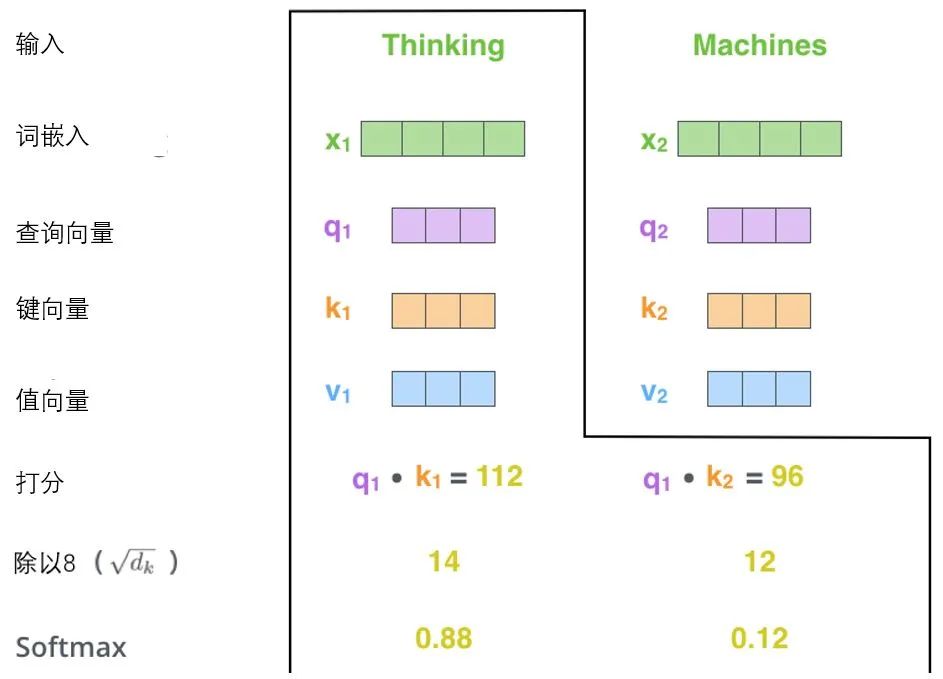
The third and fourth steps involve dividing the scores by 8 (8 is the square root of the dimension of the key vector used in the paper, which is 64, making the gradients more stable. Other values can also be used; 8 is just the default value), and then passing the results through softmax.
The role of softmax is to normalize the scores of all words, resulting in positive values that sum to 1.
This softmax score determines each word’s contribution to the encoding of the current position (“Thinking”). Obviously, words already present at this position will receive the highest softmax score, but sometimes it is also helpful to pay attention to another word that is semantically related to the current word.
The fifth step is to multiply each value vector by the softmax score (this is to prepare them for summation later). The intuition here is to focus on semantically related words and weaken irrelevant words (for example, multiplying them by a small decimal like 0.001).
The sixth step is to sum the weighted value vectors (another explanation of self-attention is that when encoding a certain word, it is to perform a weighted sum of the representations (value vectors) of all words, where the weights are obtained through the dot product of the representation of the word being encoded (query vector) and the representation of the word being processed (key vector)), and then we get the output of the self-attention layer at that position (in our example, for the first word).
Thus, the calculation of self-attention is complete. The resulting vector can be passed to the feed-forward neural network. However, in practice, these calculations are done in matrix form for faster computation. Now let’s see how it is implemented using matrices.
Implementing Self-Attention Mechanism via Matrix Operations:
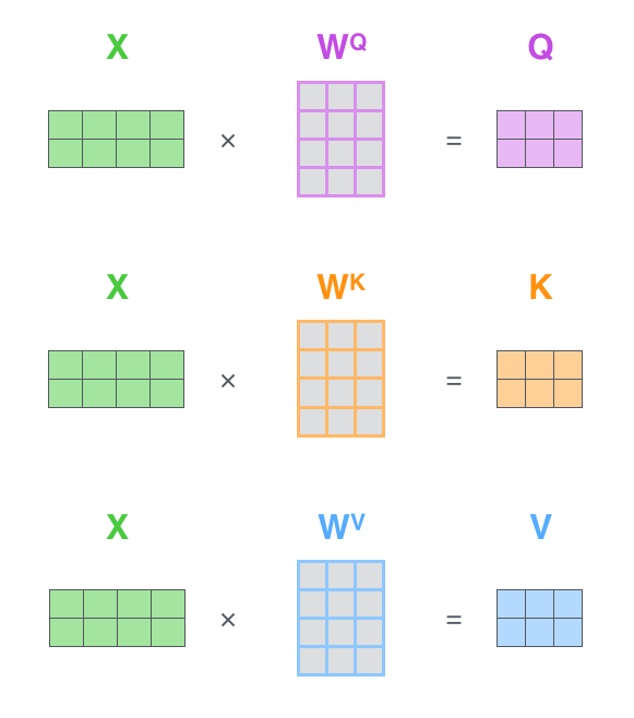
The first step is to calculate the query matrix, key matrix, and value matrix. To do this, we will put the word embeddings of the input sentence into a matrix X and multiply it by our trained weight matrices (WQ, WK, WV).
Each row in the x matrix corresponds to a word in the input sentence. We see again the size difference between the word embedding vector (512, or the 4 boxes in the image) and the q/k/v vectors (64, or the 3 boxes in the image).
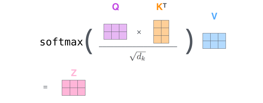
Finally, since we are dealing with matrices, we can combine steps 2 to 6 into a single formula to compute the output of the self-attention layer.
The matrix operation form of self-attention:
“Battling Multi-Headed Monsters”
By adding a mechanism called “multi-headed” attention, the paper further refines the self-attention layer and improves the performance of the attention layer in two ways:
1. It extends the model’s ability to focus on different positions. In the example above, although each encoding has more or less representation in z1, it may be dominated by the actual words themselves.
If we translate a sentence, for example, “The animal didn’t cross the street because it was too tired”, we want to know which word “it” refers to, and at this point, the model’s “multi-headed” attention mechanism comes into play.
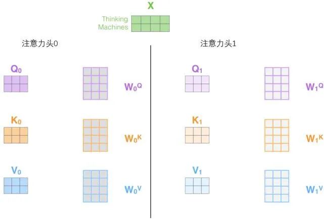
2. It provides multiple “representation subspaces” for the attention layer. Next, we will see that for the “multi-headed” attention mechanism, we have multiple sets of query/key/value weight matrices (the Transformer uses eight attention heads, so we have eight sets of matrices for each encoder/decoder).
Each of the sets in this collection is randomly initialized, and after training, each set is used to project the input word embeddings (or vectors from the lower encoders/decoders) into different representation subspaces.
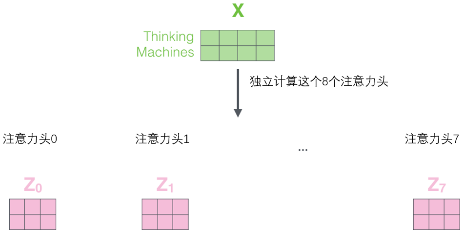
In the “multi-headed” attention mechanism, we maintain independent query/key/value weight matrices for each head, thus producing different query/key/value matrices. As before, we multiply X by the WQ/WK/WV matrices to produce the query/key/value matrices.
If we perform the same self-attention calculations as above, using eight different weight matrix operations, we will obtain eight different Z matrices.
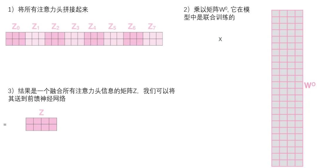
This presents a bit of a challenge. The feed-forward layer does not need eight matrices; it only needs one matrix (composed of the representation vectors for each word). So we need a way to compress these eight matrices into a single matrix.
How do we do that? In fact, we can directly concatenate these matrices together and then multiply them by an additional weight matrix WO.
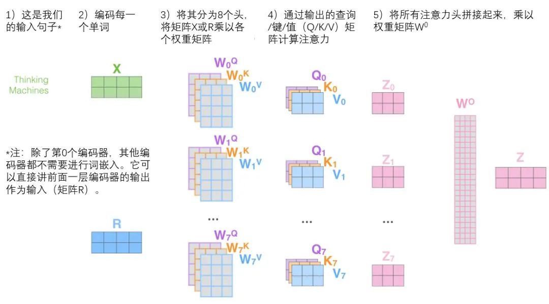
This is almost everything about multi-headed self-attention. There are indeed a lot of matrices, and we try to concentrate them in one image so that it can be seen at a glance.
Now that we have touched on so many “heads” of the attention mechanism, let’s revisit the previous example and see where different attention “heads” focus when encoding the word “it”:
When encoding the word “it”, one attention head focuses on “animal”, while another focuses on “tired”, meaning that the model’s representation of the word “it” is to some extent a representation of both “animal” and “tired”.
However, if we add all the attention to the illustration, it becomes even harder to explain:
Using Positional Encoding to Represent the Order of Sequences:
So far, our description of the model lacks a way to understand the order of input words.
To solve this problem, the Transformer adds a vector for each input word embedding. These vectors follow a specific pattern learned by the model, which helps determine each word’s position or the distance between different words in the sequence.
The intuition here is that adding positional vectors to word embeddings allows them to better express the distance between words in subsequent calculations.
To help the model understand the order of words, we add positional encoding vectors, whose values follow a specific pattern.
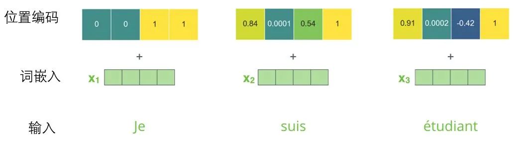
If we assume the dimensionality of the word embeddings is 4, the actual positional encoding is as follows:
Mini Word Embedding Positional Encoding Example with Dimension 4:
What would this pattern look like?
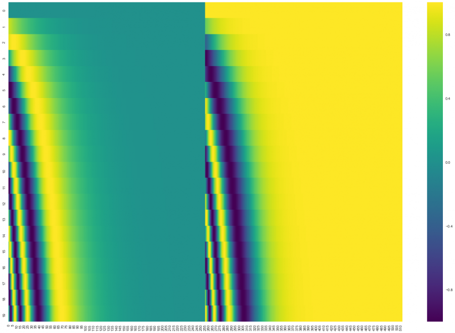
In the figure below, each row corresponds to the positional encoding of a word vector, so the first row corresponds to the first word in the input sequence. Each row contains 512 values, each value ranging between 1 and -1. We have color-coded them so that the pattern is visible.
Example of positional encoding for 20 words (rows), with a word embedding size of 512 (columns). You can see that it splits into two halves. This is because the left half’s values are generated by one function (using sine), and the right half by another function (using cosine). They are then concatenated together to obtain each positional encoding vector.
The original paper describes the formula for positional encoding (Section 3.5). You can see the code for generating positional encodings in get_timing_signal_1d(). This is not the only possible method for positional encoding.
However, its advantage is that it can scale to unknown sequence lengths (for example, when the trained model needs to translate sentences much longer than those in the training set).
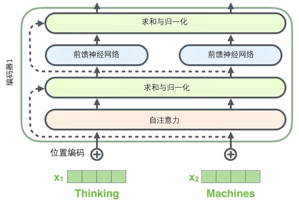
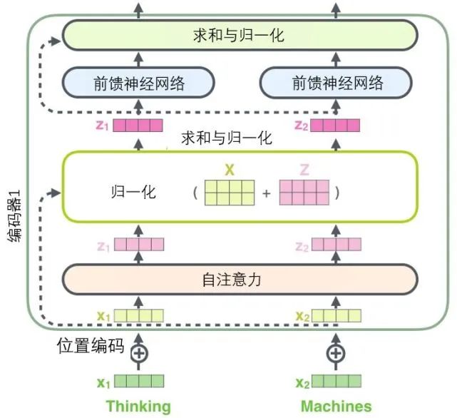
Before we continue, we need to mention a detail in the encoder architecture: there is a residual connection around each sub-layer (self-attention, feed-forward network) in each encoder, followed by a “layer normalization” step.
Layer Normalization Step:
https://arxiv.org/abs/1607.06450
If we visualize these vectors along with the layer normalization operation associated with self-attention, it looks like the diagram below describes:
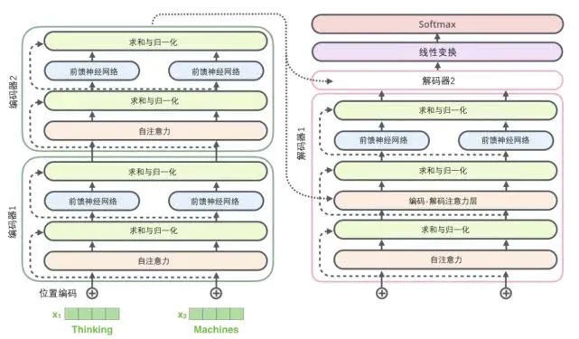
The sub-layers of the decoder are similarly structured. If we imagine a transformer structure with 2 layers of encoding and decoding, it would look like the diagram below:
Now that we have discussed most of the concepts of the encoder, we basically understand how the decoder works. But it’s best to look at the details of the decoder.
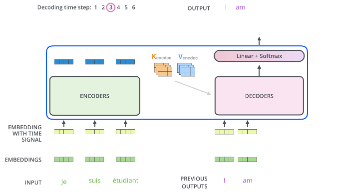
The encoder starts working by processing the input sequence. The output of the top encoder is then transformed into a set of attention vectors containing the key vectors (K) and value vectors (V).
These vectors will be used by each decoder for its own “encoder-decoder attention layer”, which can help the decoder focus on the appropriate positions in the input sequence:
After completing the encoding phase, the decoding phase begins. Each step of the decoding phase outputs an element of the output sequence (in this case, the English translation sentence).
The following steps repeat this process until reaching a special termination symbol that indicates that the transformer’s decoder has completed its output. The output of each step is provided to the bottom decoder at the next time step, and just as the encoders did before, these decoders will output their decoding results.
Additionally, just as we did with the inputs of the encoders, we will embed and add positional encodings to those decoders to represent the position of each word.
In those decoders, the behavior of the self-attention layers differs from that of the encoders: in the decoders, the self-attention layers are only allowed to process positions that are earlier in the output sequence. Before the softmax step, it will mask the later positions (setting them to -inf).
The “encoder-decoder attention layer” works similarly to the multi-headed self-attention layer, except it creates a query matrix from the layer below and retrieves the key/value matrices from the output of the encoder.
Final Linear Transformation and Softmax Layer:
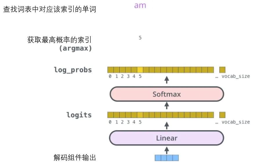
The decoder component will ultimately output a real-valued vector. How do we turn floating-point numbers into a word? That is the job of the linear transformation layer, which is followed by the softmax layer.
The linear transformation layer is a simple fully connected neural network that can project the vector produced by the decoder component into a much larger vector known as the logits.
Let’s assume our model has learned ten thousand different English words from the training set (our model’s “output vocabulary”). Therefore, the logits vector is a vector of length ten thousand, with each cell corresponding to the score of a specific word.
The subsequent softmax layer converts those scores into probabilities (all positive numbers, with an upper limit of 1.0). The cell with the highest probability is selected, and the corresponding word is output as the result for that time step.
This image starts with the output vector produced by the decoder component. It then transforms it into an output word.
Now that we have gone through the complete forward propagation process of the transformer, we can intuitively understand its training process.
During training, an untrained model goes through exactly the same forward propagation. But because we train it with a labeled training set, we can compare its output with the actual output.
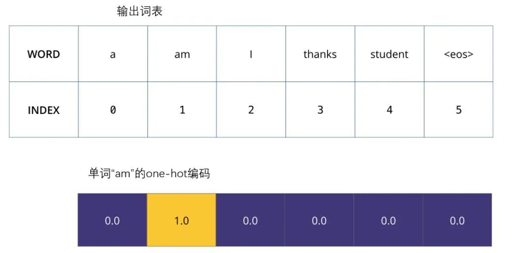
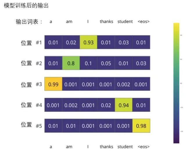
To visualize this process, let’s assume our output vocabulary only contains six words: “a”, “am”, “i”, “thanks”, “student”, and “” (the abbreviation for end of sentence).
The output vocabulary of our model has been set in the preprocessing process before we train.
Once we define our output vocabulary, we can use a vector of the same width to represent each word in our vocabulary. This is also considered a one-hot encoding. So we can use the following vector to represent the word “am”:
Example: One-hot encoding for our output vocabulary
Next, we discuss the model’s loss function – this is the standard we use to optimize during training. It allows us to train a model that produces results as accurately as possible.
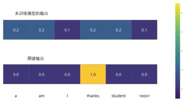
For example, we are training the model, and now it is the first step – a simple example – translating “merci” to “thanks”.
This means we want an output that represents the probability distribution of the word “thanks”. However, since this model has not been trained yet, it is unlikely to produce this result right now.
Because the parameters (weights) of the model are randomly generated, the (untrained) model produces a probability distribution with random values in each cell/word. We can compare this with the actual output and use the backpropagation algorithm to slightly adjust all model weights to generate outputs closer to the result.
How would you compare two probability distributions? We can simply subtract one from the other. For more details, please refer to cross-entropy and KL divergence.
https://colah.github.io/posts/2015-09-Visual-Information/
https://www.countbayesie.com/blog/2017/5/9/kullback-leibler-divergence-explained
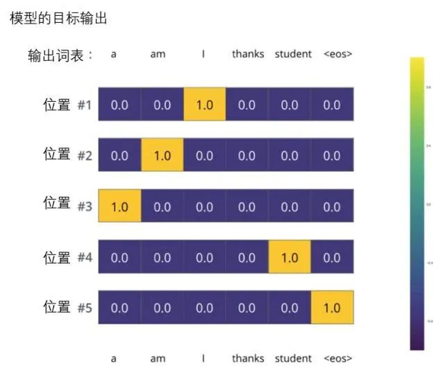
But note that this is an overly simplified example. A more realistic situation is processing a sentence. For instance, input “je suis étudiant” and expect the output to be “i am a student”. We want our model to successfully output probability distributions in these cases:
Each probability distribution is represented by a vector with a width equal to the size of the vocabulary (in our example, it is 6, but in reality, it is usually 3000 or 10000).
The first probability distribution has the highest probability in the cell associated with “i”
The second probability distribution has the highest probability in the cell associated with “am”
And so on, the fifth output distribution indicates the cell associated with “” has the highest probability.
Target probability distributions obtained from training the model based on the example:
After sufficiently training on a large dataset, we hope that the probability distributions output by the model look like this:
We expect that after training, the model will output the correct translation. Of course, if this sentence comes entirely from the training set, it is not a very good evaluation metric (reference: cross-validation, linkhttps://www.youtube.com/watch?v=TIgfjmp-4BA).
Note that each position (word) receives a bit of probability, even if it is unlikely to be the output at that time step – this is a useful property of softmax that helps the model train.
Because this model generates one output at a time, let’s assume that this model only selects the word with the highest probability and discards the rest. This is one method (called greedy decoding).
Another method to accomplish this task is to keep the two highest probability words (for example, I and a), then run the model twice in the next step: once assuming the first position’s output is the word “I”, and the other assuming the first position’s output is the word “me”, and whichever version produces less error will retain the highest probability translation results.
We repeat this step for the second and third positions. This method is called beam search (in our example, the beam width is 2, because we retained the results of two beams, such as the first and second positions), and it ultimately returns the results of two beams (top_beams is also 2). These are all parameters that can be set in advance.
Furthermore, I hope that through the above text, you have gained an understanding of the main concepts of the Transformer. If you want to delve deeper into this field, I suggest following these steps: read Attention Is All You Need, the Transformer blog, and the Tensor2Tensor announcement, and check out Łukasz Kaiser’s introduction to understand the model and details.
https://ai.googleblog.com/2017/08/transformer-novel-neural-network.html
Tensor2Tensor Announcement:https://ai.googleblog.com/2017/06/accelerating-deep-learning-research.html
Łukasz Kaiser’s Introduction:
https://colab.research.google.com/github/tensorflow/tensor2tensor/blob/master/tensor2tensor/notebooks/hello_t2t.ipynb
Future Research Directions:
Depthwise Separable Convolutions for Neural Machine Translation
https://arxiv.org/abs/1706.03059
One Model To Learn Them All
https://arxiv.org/abs/1706.05137
Discrete Autoencoders for Sequence Models
https://arxiv.org/abs/1801.09797
Generating Wikipedia by Summarizing Long Sequences
https://arxiv.org/abs/1801.10198
https://arxiv.org/abs/1802.05751
Training Tips for the Transformer Model
https://arxiv.org/abs/1804.00247
Self-Attention with Relative Position Representations
https://arxiv.org/abs/1803.02155
Fast Decoding in Sequence Models using Discrete Latent Variables
https://arxiv.org/abs/1803.03382
Adafactor: Adaptive Learning Rates with Sublinear Memory Cost
https://arxiv.org/abs/1804.04235
Original link:
https://jalammar.github.io/illustrated-transformer/
Copyright statement: This article is an original piece by the author, following the CC 4.0 BY-SA copyright agreement. Please include the original source link and this statement when reprinting.
Article link:
https://blog.csdn.net/longxinchen_ml/article/details/86533005