
This article contains about 3300 words, and is recommended to be read in 10minutes
This article introduces how to use XGBoost for time series forecasting, including transforming time series into a supervised learning prediction problem, using forward validation for model evaluation, and providing actionable code examples.
For classification and regression problems, XGBoost is an efficient implementation of the gradient boosting algorithm.
It balances speed and efficiency, and performs excellently in many predictive modeling tasks, being favored by winners in data science competitions such as Kaggle.
XGBoost can also be used for time series forecasting, although the time series dataset needs to be converted into a format suitable for supervised learning. It also requires a specialized technique for model evaluation called forward validation, as model evaluation using k-fold cross-validation can yield biased results.
In this article, you will learn how to develop an XGBoost model for time series forecasting.
By the end of this tutorial, you will know:
-
XGBoost is an implementation of the gradient boosting ensemble method for classification and regression problems.
-
By using a sliding time window representation, time series datasets can be adapted for supervised learning.
-
How to fit, evaluate, and predict with the XGBoost model on time series forecasting problems.

This tutorial is divided into three parts:
2. Time Series Data Preparation
3. XGBoost for Time Series Forecasting
XGBoost stands for Extreme Gradient Boosting, which is an efficient implementation of stochastic gradient boosting.
Stochastic gradient boosting (or gradient boosting machines or tree boosting) is a powerful machine learning technique that performs very well on many challenging machine learning problems, often achieving the best results.
Tree boosting has been shown to give state-of-the-art results on many standard classification benchmarks.
— XGBoost: A Scalable Tree Boosting System, 2016.
https://arxiv.org/abs/1603.02754
It is an ensemble of decision tree algorithms where new trees can correct the results of existing trees in the model. We can continue to add decision trees until we achieve satisfactory results.
XGBoost is an efficient implementation of the stochastic gradient boosting algorithm, which can control the model throughout the training process through a series of hyperparameters.
The most important factor behind the success of XGBoost is its scalability in all scenarios. The system runs more than ten times faster than existing popular solutions on a single machine and scales to billions of examples in distributed or memory-limited settings.
— XGBoost: A Scalable Tree Boosting System, 2016.
https://arxiv.org/abs/1603.02754
XGBoost is designed for classification and regression problems with tabular datasets and can also be used for time series forecasting.
For more information on GDBT and XGBoost implementations, see the following tutorial:
A Brief Overview of Gradient Boosting Algorithms in Machine Learning
Link: https://machinelearningmastery.com/gentle-introduction-gradient-boosting-algorithm-machine-learning/
First, XGBoost needs to be installed, which you can do using pip as follows:

After installation, you can confirm whether it was successful and check the installed version using the following code:

Executing the above code will display the version number, which may also be higher:

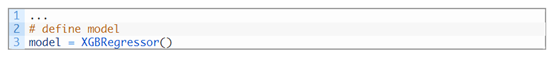
Although the XGBoost library has its own Python interface, you can also use the XGBRegressor wrapper class from the scikit-learn API.
An instance of the model can be instantiated and used for model evaluation just like any other scikit-learn class. For example:
Now that we are familiar with XGBoost, let’s look at how to prepare the time series dataset for supervised learning.
2. Time Series Data Preparation
Time data can be used for supervised learning.
Given a series of numbers from a time series dataset, we can reconstruct the data to look like a supervised learning problem. We can use the data from the previous time step as input variables and the next time step as output variables.
Let’s learn this concretely with an example. Suppose we have a set of time series data like this:
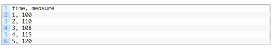
We can reshape this time series dataset into a supervised learning format, using the values from the previous time step to predict the value at the next time step.
By reorganizing the time series dataset in this way, the data will look like this:

Note! We have removed the time column, and there are several rows of data that cannot be used for training, such as the first and last rows.
This representation is called a sliding window, as the input and expected output windows move forward in time, creating new “samples” for the supervised learning model.
For more information on the sliding window method for preparing time series forecasting data, see the tutorial:
Time Series Forecasting as Supervised Learning
Link: https://machinelearningmastery.com/time-series-forecasting-supervised-learning/
You can use the shift() method from the pandas library to transform the time series data into a new framework according to the given input-output lengths.
This will be a useful tool as it allows us to explore different frameworks for time series problems with machine learning algorithms to see which method may yield better models.
The following function takes a time series as a NumPy array with one or more columns and converts it into a supervised learning problem with a specified number of inputs and outputs.
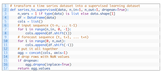
We can use this function to prepare a time series dataset for XGBoost.
For more information on the step-by-step development of this function, see the tutorial:
How to Convert Time Series into Supervised Learning Problems in Python
Link: https://machinelearningmastery.com/convert-time-series-supervised-learning-problem-python/
Once the dataset is prepared, we need to focus on how to use it to fit and evaluate a model.
For example, a model that predicts historical data using future data is invalid. The model must predict the future based on historical data.
This means that during the model evaluation phase, methods like random splitting of datasets similar to k-fold cross-validation are not applicable. Instead, we must use a technique called forward validation.
In forward validation, the data is first split into a training set and a test set by selecting a split point, such as removing the last 12 months of data for training and using the last 12 months of data for testing.
If we are interested in a one-step prediction, such as one month, we can evaluate the model by training on the training dataset and predicting the first time step in the test dataset. Then, we can add the actual observations from the test set to the training dataset, retrain the model, and let the model predict the second time step in the test dataset.
Repeating this process across the entire test set allows us to obtain one-step predictions and calculate the error rate to evaluate the model’s performance.
For more information on forward validation, see the tutorial:
How To Backtest Machine Learning Models for Time Series Forecasting
Link: https://machinelearningmastery.com/backtest-machine-learning-models-time-series-forecasting/
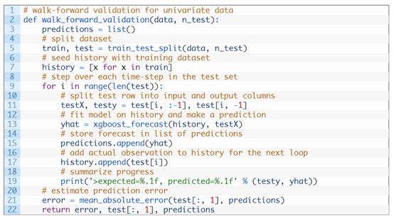
The function below runs forward validation.
The parameters are the entire time series dataset and the number of rows to use for the test set.
Then it iterates through the test set, calling the xgboost_forecast() function to make one-step predictions. It calculates error metrics and returns details for analysis.
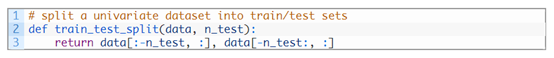
The train_test_split() function is used to split the dataset into training and testing sets. This method can be defined as follows:
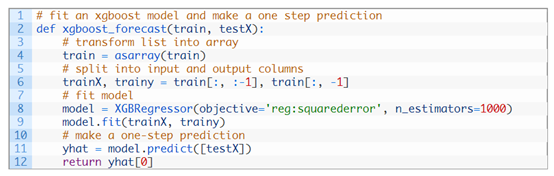
The XGBRegressor class can be used for one-step predictions. The xgboost_forecast() method implements fitting the model using the training and test set inputs, and then making one-step predictions.
Now that we know how to prepare the time series dataset for forecasting and evaluate the XGBoost model, we can use XGBoost on real datasets.
3. XGBoost for Time Series Forecasting
In this section, we will explore how to use XGBoost for time series forecasting.
We will use a standard univariate time series dataset, aiming to make one-step predictions with the model.
You can use the code from this section to start your own project, and it can easily be adapted for multivariate inputs, multivariate predictions, and multi-step predictions.
The following links can be used to download the dataset, which can be imported into your local working directory as “daily-total-female-births.csv”.
-
Dataset (daily-total-female-births.csv)
Link: https://raw.githubusercontent.com/jbrownlee/Datasets/master/daily-total-female-births.csv
-
Description (daily-total-female-births.names)
Link: https://raw.githubusercontent.com/jbrownlee/Datasets/master/daily-total-female-births.names
The first few rows of the dataset are shown below:

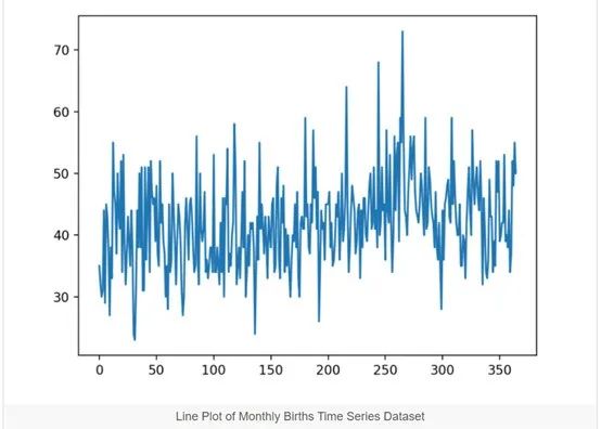
First, import the data and plot the dataset. The complete example is as follows:
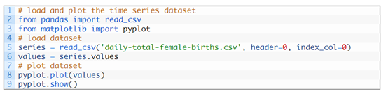
Running this example will produce a line plot of the dataset. It can be observed that there is no obvious trend or seasonality.
In the problem of predicting the number of births in the next 12 months, the persistence model achieved an average absolute error (MAE) of 6.7. This provides a valid benchmark for the model.
Next, we evaluate the performance of the XGBoost model on this dataset and make one-step predictions on the last 12 months of data.
We only use the first three time steps as model inputs and the default model hyperparameters, but we change the loss to ‘reg:squarederror’ (to avoid warning messages) and use 1000 trees in the ensemble (to avoid underfitting).
The complete example is as follows:
# forecast monthly births with xgboost
from numpy import asarray
from pandas import read_csv
from pandas import DataFrame
from pandas import concat
from sklearn.metrics import mean_absolute_error
from xgboost import XGBRegressor
from matplotlib import pyplot
# transform a timeseries dataset into a supervised learning dataset
def series_to_supervised(data, n_in=1, n_out=1, dropnan=True):
n_vars = 1 if type(data) is list else data.shape[1]
df = DataFrame(data)
cols = list()
# input sequence (t-n, ... t-1)
for i in range(n_in, 0, -1):
cols.append(df.shift(i))
# forecast sequence (t, t+1, ... t+n)
for i in range(0, n_out):
cols.append(df.shift(-i))
# put it all together
agg = concat(cols, axis=1)
# drop rows with NaN values
if dropnan:
agg.dropna(inplace=True)
return agg.values
# split a univariate dataset into train/test sets
def train_test_split(data, n_test):
return data[:-n_test, :], data[-n_test:, :]
# fit an xgboost model and make a one step prediction
def xgboost_forecast(train, testX):
# transform list into array
train = asarray(train)
# split into input and output columns
trainX, trainy = train[:, :-1], train[:, -1]
# fit model
model = XGBRegressor(objective='reg:squarederror', n_estimators=1000)
model.fit(trainX, trainy)
# make a one-step prediction
yhat = model.predict(asarray([testX]))
return yhat[0]
# walk-forward validation for univariate data
def walk_forward_validation(data, n_test):
predictions = list()
# split dataset
train, test = train_test_split(data, n_test)
# seed history with training dataset
history = [x for x in train]
# step over each time-step in the test set
for i in range(len(test)):
# split test row into input and output columns
testX, testy = test[i, :-1], test[i, -1]
# fit model on history and make a prediction
yhat = xgboost_forecast(history, testX)
# store forecast in list of predictions
predictions.append(yhat)
# add actual observation to history for the next loop
history.append(test[i])
# summarize progress
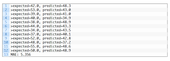
print('>expected=%.1f, predicted=%.1f' % (testy, yhat))
# estimate prediction error
error = mean_absolute_error(test[:, 1], predictions)
return error, test[:, 1], predictions
# load the dataset
series = read_csv('daily-total-female-births.csv', header=0, index_col=0)
values = series.values
# transform the timeseries data into supervised learning
data = series_to_supervised(values, n_in=3)
# evaluate
mae, y, yhat = walk_forward_validation(data, 12)
print('MAE: %.3f' % mae)
# plot expected vs predicted
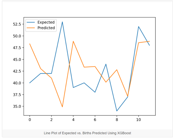
pyplot.plot(y, label='Expected')
pyplot.plot(yhat, label='Predicted')
pyplot.legend()
pyplot.show()
Running this example will report the expected and predicted values for each time in the test set, and then report the MAE for all predictions.
We can see that the model performs better than the persistence model with an MAE of about 5.3 births.
You can try different XGBoost hyperparameters and different time step inputs to see if you can achieve a better model. Feel free to share your results in the comments section.
The following figure shows a line plot comparing the predicted values and actual values for the last 12 months, providing a visual representation of the model’s performance on the test set.
Once the final XGBoost model parameters are selected, a model can be determined and used to make predictions on new data.
This is called out-of-sample prediction, such as predicting beyond the training set. This is the same as making predictions during model evaluation: because the process of evaluating which model to select and making predictions with that model on new data is identical.
The following example demonstrates how to fit the final XGBoost model on all available data and make one-step predictions beyond the end of the dataset.
# finalize model and make a prediction for monthly births with xgboost
from numpy import asarray
from pandas import read_csv
from pandas import DataFrame
from pandas import concat
from xgboost import XGBRegressor

# transform a timeseries dataset into a supervised learning dataset
def series_to_supervised(data, n_in=1, n_out=1, dropnan=True):
    n_vars = 1 if type(data) is list else data.shape[1]
    df = DataFrame(data)
    cols = list()
    # input sequence (t-n, ... t-1)
    for i in range(n_in, 0, -1):
        cols.append(df.shift(i))
    # forecast sequence (t, t+1, ... t+n)
    for i in range(0, n_out):
        cols.append(df.shift(-i))
    # put it all together
    agg = concat(cols, axis=1)
    # drop rows with NaN values
    if dropnan:
        agg.dropna(inplace=True)
    return agg.values

# load the dataset
series = read_csv('daily-total-female-births.csv', header=0, index_col=0)
values = series.values

# transform the timeseries data into supervised learning
train = series_to_supervised(values, n_in=3)

# split into input and output columns
trainX, trainy = train[:, :-1], train[:, -1]

# fit model
model = XGBRegressor(objective='reg:squarederror', n_estimators=1000)
model.fit(trainX, trainy)

# construct an input for a new prediction
row = values[-3:].flatten()

# make a one-step prediction
yhat = model.predict(asarray([row]))
print('Input: %s, Predicted: %.3f' % (row, yhat[0]))
Running this code will build an XGBoost model based on all available data.
Using the last three months of known data as the new input row, it predicts the next month after the end of the dataset.

If you want to delve deeper, this section will provide more resources on the topic.
-
A Brief Introduction to Gradient Boosting Algorithms in Machine Learning
https://machinelearningmastery.com/gentle-introduction-gradient-boosting-algorithm-machine-learning/
-
Time Series Forecasting as a Supervised Learning Problem
https://machinelearningmastery.com/time-series-forecasting-supervised-learning/
-
How to Convert Time Series Problems into Supervised Learning Problems in Python
https://machinelearningmastery.com/convert-time-series-supervised-learning-problem-python/
-
How To Backtest Machine Learning Models for Time Series Forecasting
https://machinelearningmastery.com/backtest-machine-learning-models-time-series-forecasting/
In this tutorial, you learned how to develop an XGBoost model for time series forecasting.
Specifically, you learned:
-
XGBoost is an implementation of the gradient boosting ensemble algorithm for classification and regression.
-
Time series datasets can be transformed into supervised learning through sliding window representation.
-
How to fit, evaluate, and predict with the XGBoost model for time series forecasting.
Original title:
How to Use XGBoost for Time Series Forecasting
Original link:
https://machinelearningmastery.com/xgboost-for-time-series-forecasting/
Wang Weili, BI practitioner in the elderly care and medical industry. Keep learning.
Translation Team Recruitment Information
Job Description: A meticulous heart is needed to translate selected foreign articles into fluent Chinese. If you are a data science/statistics/computer science student studying abroad, or working overseas in related fields, or confident in your language skills, welcome to join the translation team.
What you can gain: Regular translation training to improve volunteers’ translation skills, enhance awareness of cutting-edge data science, overseas friends can stay in touch with domestic technical application development, and the THU Data Team’s background provides good development opportunities for volunteers.
Other Benefits: Data science workers from well-known companies, students from prestigious universities such as Peking University and Tsinghua University, as well as overseas students, will become your partners in the translation team.
Click the “Read Original” at the end of the article to join the Data Team~
Reprint Notice
If you need to reprint, please indicate the author and source prominently at the beginning (reprinted from: Data Team ID: DatapiTHU), and place a prominent QR code for Data Team at the end of the article. For articles with original identification, please send [Article Name – Authorized Public Account Name and ID] to the contact email to apply for whitelist authorization and edit according to requirements.
After publishing, please feedback the link to the contact email (see below). Unauthorized reprints and adaptations will be pursued legally.

Click “Read Original” to embrace the organization