
As China’s economy and society rapidly develop, the living standards of the people continue to improve, and the public’s attention to food safety is increasingly heightened.[1] In food safety risk management, food safety risk assessment is a powerful means of analyzing and solving food safety problems based on data. The Food Safety Law of the People’s Republic of China, implemented in 2009, stipulates that “the state establishes a food safety risk monitoring system, and the Ministry of Health, in conjunction with the State Administration for Market Regulation and other departments, formulates and implements a national food safety risk monitoring plan and establishes a food safety risk assessment expert committee composed of experts in medicine, agriculture, food, nutrition, biology, and environment to conduct food safety risk assessments.”[2]This regulation emphasizes the significant practical importance of conducting food safety risk assessments and predictions.
Currently, risk assessment methods mainly include subjective weighting evaluation methods, objective weighting evaluation methods, and comprehensive subjective-objective weighting evaluation methods. Among subjective weighting evaluation methods, Analytic Hierarchy Process (AHP) and Delphi methods are currently the more mature risk assessment methods. AHP addresses complex multi-objective decision-making problems by constructing a three-layer structure of goal layer, criterion layer, and alternative layer[3], but still has deficiencies such as structural complexity and susceptibility to the influence of authoritative figures[4]; the Delphi method is a feedback anonymous inquiry method relying on numerous expert opinions[5], which obtains consistent opinions through continuous integration, summarization, and statistics, but the process of collecting and summarizing expert opinions is relatively complex and time-consuming[6]. Among objective weighting evaluation methods, algorithms such as back propagation (BP), random forest (RF), and support vector machine (SVM) are widely used. The BP algorithm[7] is a fast gradient descent algorithm with strong nonlinear mapping capabilities, but it is prone to local minimum problems; the RF algorithm[8] is an extended variant of Bagging with low computational complexity, but it is prone to overfitting; the SVM algorithm[9] has strong generalization capabilities but is not suitable for large datasets. The comprehensive subjective-objective weighting evaluation method builds an indicator system through subjective weighting evaluation and constructs a risk prediction model based on objective weighting evaluation to achieve precise and efficient risk assessment.
Existing risk evaluation methods still have certain limitations in practical applications[10], such as high labor costs for subjective analysis and long evaluation processes, as well as low precision of evaluation indicators or weak overfitting performance for objective analysis, resulting in low accuracy and high time costs for risk prediction results, which leads to a lack of ability to accurately locate risk values. Therefore, in response to the characteristics of the food industry, this study introduces maximum residue limits (MRL) and acceptable daily intake (ADI) of contaminants for quantitative improvement of AHP and combines it with the XGBoost algorithm, which has high prediction accuracy and is less prone to overfitting, to construct a prediction model for application in food safety risk assessment. Through case analysis based on rice testing data from 31 provinces in mainland China, the improved AHP model extracts comprehensive feature values from multidimensional complex data as risk values for the prediction model, and the stable and high-precision XGBoost algorithm is used as the training model for risk value prediction, while the same data is applied to classical prediction algorithms for comparison to verify the effectiveness of the XGBoost algorithm.

1.1 Data Source
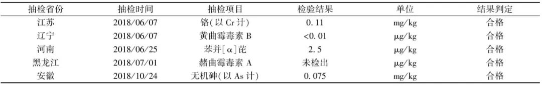
The analysis is based on the 2018 rice contaminant testing data. By collecting and integrating data from the National Food Safety Sampling Inspection Information System, testing data for rice contaminants from 31 provinces and cities in mainland China, excluding Hong Kong, Macao, and Taiwan, was obtained. This data primarily consists of categories such as sampling province, sampling time, sampling items, and inspection results, where the contaminant testing items include total mercury, inorganic arsenic, lead, chromium, cadmium, aflatoxin B, and other contaminants, with some data shown in Table 1.
Table 1 Original Data of Rice Contaminant Testing in 2018
1.2 Data Cleaning
For the contaminant testing data collected in section 1.1, in order to extract effective information from high-dimensional complex data and achieve the transformation of data value from implicit to explicit[11], this study sequentially employs data filtering, data reduction, and data transformation methods to clean the original data, as shown in Figure 1.
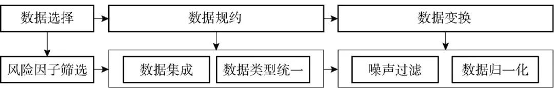
Figure 1 Data Cleaning Process
1.2.1 Risk Factor Screening
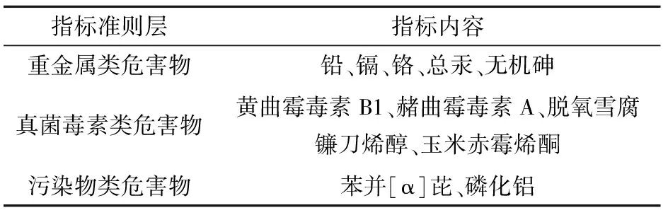
Risk factors refer to non-intentionally added chemical hazardous substances that are generated during the production, processing, packaging, storage, transportation, sale, and consumption of rice, or introduced by environmental pollution[12-13]. The screening process is as follows: 1) Classify the testing results based on their attributes. The testing results for each contaminant are divided into descriptive results, numerical results, and null values, where descriptive results primarily include undetected or below a specific value (e.g., <0.01 μg/kg), and numerical results are specific detected amounts (e.g., 0.11 μg/kg). 2) Convert descriptive results to numerical results. Since numerical results can more intuitively reflect the level of contaminants compared to descriptive results, unnecessary symbols are deleted for descriptive results below a specific value. For example, aflatoxin B detection content of “<0.001 μg/kg” is recorded as “0.001 μg/kg” as it does not exceed the national standard limit of 10 μg/kg; if aflatoxin A is undetected, it is recorded as “0 μg/kg.” 3) Count the number of numerical results for each contaminant and the number of contaminants exceeding national limit values. The contaminants are arranged in descending order based on the ratio of the number of contaminants exceeding national limit values to the number of numerical results, selecting those with a larger ratio as risk factors. Based on the screening process, a risk indicator system for rice contaminants is constructed, as shown in Table 2.
Table 2 Risk Indicator System for Rice Contaminants
1.2.2 Data Reduction
Data reduction mainly includes two steps: data integration and unification of data types. Data integration refers to logically integrating data with different attributes or formats; data type unification means unifying all numerical data into floating-point format for easier management.
1.2.3 Data Transformation
Data transformation also consists of noise filtering and data normalization. Noise filtering refers to removing unexplained data fluctuations, i.e., deleting missing values and removing outliers. Since the original data’s test results and result units are in a separate parallel state, the outliers in this study are statistical errors caused by incorrect unit records, i.e., values exceeding 500 times the mean of all original data.
At the same time, to ensure the quality of risk factor input, the data is normalized, i.e., mapped to a specific data space according to an appropriate membership curve. In this study, a trapezoidal membership function is used, as shown in Equation (1).
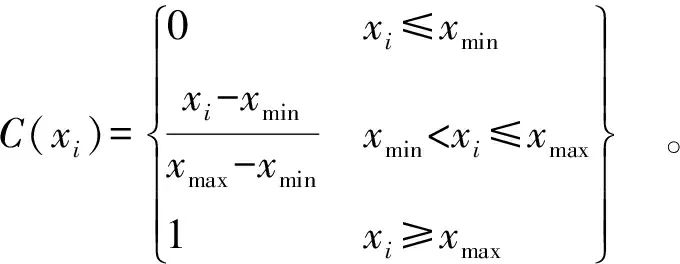
(1)
In Equation (1), xmin is the maximum value without risk, where no risk means that the detection value of the risk factor is significantly lower than the national limit value, so the percentage of the national limit value is selected as the maximum value without risk; xmax is the national limit value. The processed data is substituted into the membership function to calculate the comprehensive feature value, which is marked as the risk value of the prediction model.

2.1 Risk Prediction Model Framework
By performing data cleaning operations on the multidimensional complex rice contaminant testing data, the risk factor indicators for rice contaminants were obtained. Based on these risk factor indicator values, an integrated risk prediction model combining improved AHP and XGBoost algorithms was constructed. Since AHP is significantly influenced by subjective factors, this study quantitatively improved it by combining ADI and MRL in consideration of the characteristics of the food safety field, while employing the high-fitting and fast XGBoost algorithm for feature learning to extract comprehensive feature values of contaminants, as shown in Figure 2.

Figure 2 Risk Prediction Model Framework
2.2 Quantitative Improvement of AHP
AHP is a systematic analysis method that integrates quantitative and qualitative analysis, allowing for scientific and systematic multi-objective decision analysis[14]. The basic idea is to calculate the weights of indicators using a scoring scale of 1 to 9 provided by experts, according to the hierarchical structure of the indicator system, thus transforming complex high-dimensional data into several low-dimensional comprehensive factors[15]. However, since expert scoring is heavily influenced by subjective factors and requires high labor costs[16], to address this issue, considering the actual residual range of food produced under good agricultural practices during consumption and the allowable residue levels, this study introduces maximum residue limits set by the World Health Organization for residues in food, using the relative weight indicators formed by combining ADI and MRL of contaminants to replace expert scoring in establishing the judgment matrix, thereby obtaining the weight values of each indicator, making them more objective compared to traditional AHP.
First, let there be k risk factors, then the indicator weights for evaluating risk factors can be expressed as matrix Nk×2[Equation (2)]:
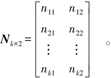
(2)
In Equation (2), ni1[i∈(1,2,…,k)] represents the ADI weight corresponding to the i-th risk factor; ni2[i∈(1,2,…,k)] represents the MRL weight corresponding to the i-th risk factor. The evaluation indicator values for the risk factors can be expressed as matrix M2×k[Equation (3)]:
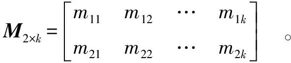
(3)
In Equation (3), m1i[i∈(1,2,…,k)] represents the ADI of the i-th risk factor; m2i[i∈(1,2,…,k)] represents the MRL of the i-th risk factor.
Combining the weight matrix for evaluating risk factors with the indicator value matrix for evaluating risk factors forms the judgment matrix Ak×k[Equation (4)], while integrating expert intervention suggestions for accuracy verification and result correction of the judgment matrix Ak×k.
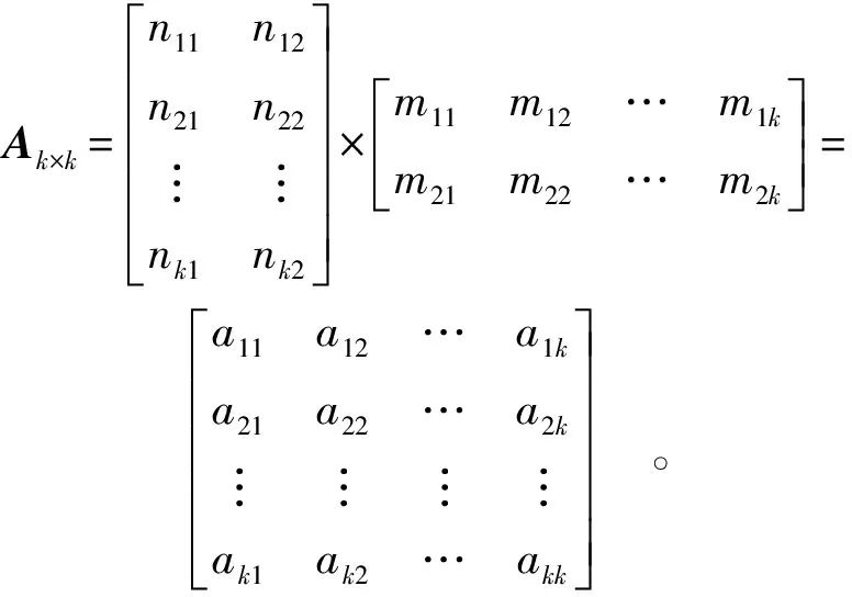
(4)
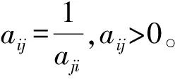
In Equation (4), the elements of matrix Ak×k correspond to the scales shown in Table 3, and it satisfies
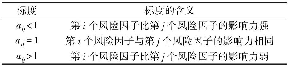
Table 3 Scales of Elements in the Judgment Matrix
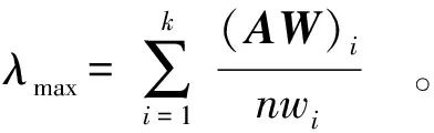
Based on the judgment matrix, the maximum eigenvalue λmax and eigenvector W=[w1,w2,…,wk]T[Equations (5) to (7)] are calculated:
AW=λmaxW;
(5)
(6)

(7)
The normalized eigenvector W is recorded as the risk factor weight value, which reflects the degree of harm of each risk factor[17]. Using the method from section 1.2 to clean and classify redundant data, a risk factor matrix X[Equation (8)] is formed, containing q data points and k dimensions:

(8)
By weighting matrix X with the weights of each risk factor indicator, a low-dimensional comprehensive risk value Y[Equation (9)] is obtained:
Y=W×XT=[w1,w2,…,wk]× 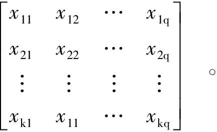
(9)
Therefore, the improved AHP model is used to reduce the dimensionality of food testing data, obtaining low-dimensional comprehensive risk values, and then using the specific quantitative indicators unique to the field of food safety risk assessment, namely MRL and ADI, as evaluation criteria to enhance the accuracy and objectivity of risk values, ultimately yielding the expected output of the rice contaminant risk prediction model.
2.3 XGBoost Algorithm Training
XGBoost algorithm[10] is a gradient boosting tree algorithm that supports parallel computing, derived from the gradient boosting decision tree (GBDT) through second-order Taylor expansion of the cost function. The XGBoost algorithm enhances both running speed and prediction accuracy while effectively suppressing overfitting[18]. The training process of the XGBoost algorithm is illustrated in Figure 3.
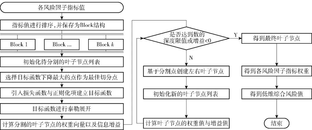
Figure 3 XGBoost Algorithm Training Process
The mathematical model can be expressed as Equations (10) and (11):
(10)
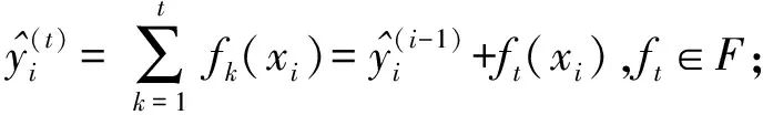
F=f(xi)=wq(x) .
(11)
In Equations (10) and (11), i∈(1,2,…,n) represents the sample number,i is the low-dimensional comprehensive risk value, xi is the value of each risk factor indicator, t is the total number of sub-models, and wq(x) is the weight vector of all leaf nodes in XGBoost, while fk is the weight of each leaf node on the k-th regression tree, and F is the collection of all regression trees.
The loss function l(yi,i)=(yi–i)2 represents the error dimension between the low-dimensional comprehensive risk value and its predicted value; the optimal solution of the loss function l(yi,i) is F*(x)=arg min E(x,y)[L(y,F(x))], which helps select the appropriate number of leaf nodes, preventing the number of leaf nodes from growing infinitely, thus effectively saving model running time; the regularization term Ω(ft)[Equation (12)] prevents the number of leaf nodes in the XGBoost algorithm from growing infinitely, speeding up model running time.

(12)
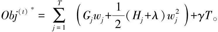
In Equation (12), γ and λ are adjustment parameters used to prevent overfitting in the model; T is the number of leaf nodes. The regularization term is positively correlated with the number of nodes; thus, introducing a regularization term can quickly derive the saturation value of leaf nodes while ensuring the stability of the error between the predicted low-dimensional comprehensive risk value and the risk value, thus improving the model’s running speed.[19].
The objective function composed of the loss function and regularization term Obj(t)[Equation (13)] is introduced:

(13)
To accelerate and improve the precision of the gradient descent of the objective function, the objective function Obj(t) is Taylor expanded to obtain the following objective function Obj(t)[Equations (14) to (17)]:
(14)
gi=∂(t-1)l(yi, (t-1));
(15)
(16)
(17)
Given this, the main contradiction of the problem is transformed into solving the minimum value problem of the following two quadratic functions [Equations (18) and (19)].
 =Gj+(Hj+λ)wj=0;
(18)
(19)
To avoid excessive computational load due to multiple enumerations, a greedy algorithm is employed to seek the optimal tree structure, adding new splits to known leaf nodes[20] and sequentially obtaining the gain from the splits, as shown in Equation (20).
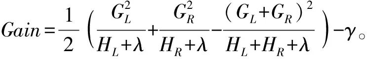
(20)
In Equation (20), Gain represents the information gain, which is the main reference factor for whether the tree structure branches. That is, when the information gain from a new split reaches the depth limit of the tree or Gain<0, the tree stops splitting, thus achieving a fast and optimal simulation effect while preventing overfitting.

3.1 Parameter Configuration of Different Models
The experimental environment of this study is a Win10 operating system with an i5-6200U CPU and 8G RAM, and the code is implemented based on the Jupyter Notebook platform using Python3. Based on this environment configuration, the indicator values selected in section 1.2 are used as input data for the risk prediction model, and the low-dimensional comprehensive risk values are used as output data. The dataset is divided according to a 3:1 training-test ratio, and the prediction results of the XGBoost algorithm model are compared with those of mainstream models with proven prediction effects, namely the k-nearest neighbor (KNN) algorithm, SVM algorithm, BP algorithm, and long short-term memory (LSTM) neural network algorithm. Since each algorithm has different parameter configurations, several parameters for each algorithm are selected using the randomized search provided by scikit-learn for parameter configuration. The parameter configuration results for each model are shown in Table 4.
Table 4 Parameter Configuration of Different Algorithms
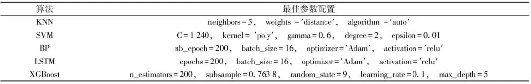
In Table 4, the best parameter configuration for the KNN algorithm consists of the number of neighbors, weight function for prediction, and the algorithm for calculating the nearest neighbors; the best parameter configuration for the SVM algorithm consists of the penalty coefficient, kernel function (kernel, gamma, degree), and distance error (epsilon), where gamma and degree are parameters inherent to the polynomial kernel function used in SVM, implicitly determining the distribution of data after mapping to the new feature space. The best parameter configuration for the BP algorithm consists of the number of iterations (nb_epoch), the number of samples selected for training at one time (batch_size), optimizer, and activation function. The best parameter configuration for the LSTM algorithm is similar to that of the BP algorithm, also consisting of the number of iterations (epochs), the number of samples selected for training at one time (batch_size), optimizer, and activation function. The best parameter configuration for the XGBoost algorithm consists of the number of iterations (n_estimators), sampling rate (subsample), random seed (random_state), learning rate (learning_rate), and maximum depth of each binary tree (max_depth).
3.2 Model Accuracy Analysis
Based on the simulation configurations in section 3.1, using different risk prediction models, with each algorithm trained for 200 iterations, the risk values of various risk factors are compared with the predicted values of different models, as shown in Figure 4. Here, the X axis represents the sample number; the Y axis represents the pollution level of various contaminants, i.e., low-dimensional comprehensive risk values. A low-dimensional comprehensive risk value greater than 1 (y>1) indicates that the pollution level exceeds 1, meaning that the contaminant is significantly over the limit; when y∈(0,1), the size of values in matrix Y is positively correlated with the pollution level of that contaminant.
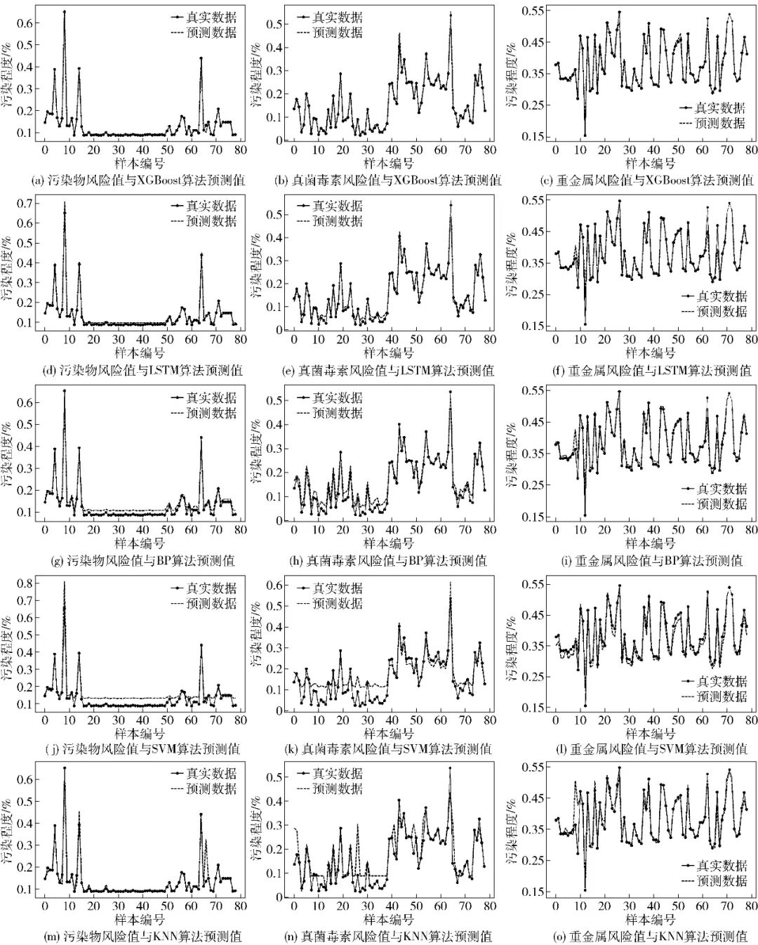
Figure 4 Comparison of Risk Values of Various Risk Factors with Different Model Predictions
From the 15 model comparison curves in Figure 4, it can be seen that when y∈(0.2,0.8), i.e., when the pollution levels of various contaminants are within a reasonable range, the predicted values of various models closely match the true values; whereas when y∈(0,0.2)∪(0.8,+∞), i.e., when the pollution levels of various contaminants are either too low or too high, some models (KNN, SVM, BP) exhibit poorer average fitting effects and tend to overestimate (or underestimate) pollution levels when they are high (or low).
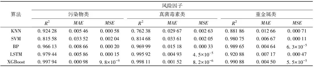
To more clearly compare the experimental results of various models, this study employs three indicators: the correlation coefficient R2, mean absolute error (MAE), and mean square error (MSE) to evaluate the models, with calculations shown in Equations (21) to (23).
(21)

(22)
(23)
In Equations (21) to (23), n represents the total number of samples, yo and ym are the true and predicted values of the low-dimensional comprehensive risk, respectively, representing the average and average predicted values of the low-dimensional comprehensive risk. The size of R2 is positively correlated with the fitting degree of the curve, while MAE and MSE are important indicators for measuring variable accuracy, with their values negatively correlated with model accuracy. The evaluation indicators of different algorithms are compared in Table 5.
Table 5 Comparison of Model Evaluation Indicators for Different Algorithms

From Table 5, it can be seen that the correlation coefficient R2 range for the XGBoost algorithm is less than one percentage point, showing particularly stable performance in predicting various contaminants, and compared to other models, the R2 of the XGBoost algorithm is generally higher, reaching over 99%. Similarly, both the MAE and MSE of the XGBoost algorithm, whether in range or value, are lower than those of other models, indicating that this model exhibits good learning ability in predicting various contaminants. In comprehensive comparison of five algorithms, the XGBoost algorithm demonstrates higher accuracy and stronger stability in predictions compared to other algorithms, thus providing a more intuitive and accurate prediction and analysis of food safety hazard risk values.

This study addresses issues such as low data utilization and high labor costs caused by high-dimensional, complex, and nonlinear food safety testing data. It comprehensively considers the specific hazardous substance limit standards in the food industry, quantitatively improves the dimensionality reduction model AHP, and combines it with the high-precision XGBoost algorithm, proposing an integrated food safety risk prediction model combining improved AHP and XGBoost algorithms. Based on this, this study processes raw data from rice contaminant testing across all provinces in mainland China, excluding Hong Kong, Macao, and Taiwan, into structured data using data reduction, data transformation, and data normalization methods. Subsequently, the quantitatively improved AHP model extracts low-dimensional comprehensive risk values, and finally, the XGBoost algorithm adaptively mines the relationship between risk factors and low-dimensional risk values. By comparing the simulation results of the model, the integrated AHP and XGBoost risk prediction model outperforms traditional risk prediction models in terms of accuracy and stability. Therefore, the establishment of the integrated improved AHP and XGBoost algorithm model can quickly and accurately identify the risk values of various contaminants, thereby providing a scientific and effective basis for decision-making by regulatory authorities; however, improvements are still needed in some aspects, such as in data application, where using a dynamic weighting method for weight allocation would better meet actual needs due to the differences in hazardous substance testing projects for various foods; and in model application, real-time monitoring of risk value changes across the entire supply chain would help reduce risks associated with food sources.


Funding Projects: Beijing Natural Science Foundation Project (4222042); National Natural Science Foundation Project (61903008); Beijing Excellent Talent Cultivation Fund Youth Top Team Project (2018000026833TD01).