
Author: milter
Link: https://www.jianshu.com/p/1405932293ea
Word2Vec has become a foundational algorithm in the field of NLP. As an AI practitioner, you should feel embarrassed if you do not actively familiarize yourself with this algorithm. This article is a translation, and the original link is: http://mccormickml.com/2016/04/19/word2vec-tutorial-the-skip-gram-model/If your English is good, I strongly recommend reading the original text directly. This article is very well written, concise, and fluent.
This is the best article I believe for getting started with Word2Vec, bar none. Of course, I am not just translating it rigidly, but rather rewriting it according to my understanding to make it clearer.
Feel free to share your thoughts in the comments, and let’s communicate more. There are two common algorithms for Word2Vec: CBOW and Skip-Gram. This article will focus on the Skip-Gram algorithm.
1Basic Idea of the Algorithm
Word2Vec, as the name implies, transforms words in the corpus into vectors for various calculations based on word vectors. The most common representation method is counting encoding. Suppose our corpus consists of the following three sentences: I like deep learning I like NLP I enjoy flying. Using counting encoding, we can draw the following matrix:
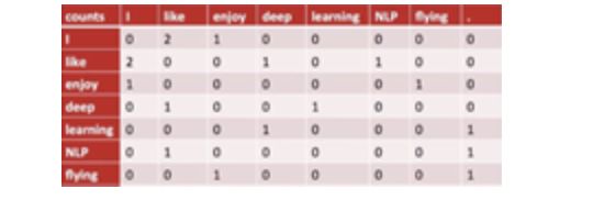
Assuming there are N words in the corpus, the size of the matrix above is N*N, where each row represents the vector representation of a word. For example, the first row 0 2 1 0 0 0 0 represents the vector for the word I. The number 2 indicates that the word I appears together with the word like in the corpus 2 times. It seems that we have simply completed “Word2Vec”, right? However, this method has at least three flaws:
-
1. When the number of words is large, the vector dimensions are high and sparse, making the vector matrix huge and difficult to store.
-
2. The vectors do not contain the semantic content of the words; they are based solely on statistical counts.
-
3. When new words are added to the corpus, the entire vector matrix needs to be updated.
Although we can reduce the dimensionality of the vectors using SVD, SVD itself is a computation-intensive operation.
Clearly, this method is not practical in real situations. The Skip-Gram algorithm we will study today successfully overcomes these three flaws. Its basic idea is to first one-hot encode all words, input them into a neural network with only one hidden layer, and train it after defining the loss.
We will explain how to define the loss later; for now, let’s put that aside. After training is complete, we can use the weights of the hidden layer as the vector representation of the words!
This idea sounds quite magical, doesn’t it? In fact, we are already familiar with it. When using an auto-encoder, we also train a neural network with one hidden layer, and after training, we discard the output layer and only use the output of the hidden layer as the final vector object, successfully completing vector compression.
2Example Explanation
1 Constructing Training Data
Suppose our corpus contains only one sentence: The quick brown fox jumps over the lazy dog. This sentence contains a total of 8 words (considering The and the as the same word).
How does the Skip-Gram algorithm generate word vectors for these 8 words? We know that training with a neural network generally involves the following steps:
-
Prepare the data, i.e., X and Y
-
Define the network structure
-
Define the loss
-
Select an appropriate optimizer
-
Conduct iterative training
-
Store the trained network
So, let’s first focus on how to determine the forms of X and Y. It’s actually very simple; (x,y) are pairs of words. For example, (the, quick) is a word pair, where the is the sample data and quick is the label for that sample.
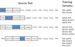
So, how do we generate word pair data from the above sentence? The answer is the n-gram method. Instead of talking too much, let’s look at the diagram:
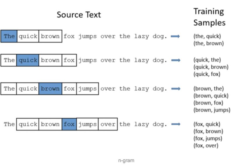
We scan the sentence word by word, and for each word we scan, we take the two words on each side (a total of 4 words) and form word pairs with the scanned word as our training data.
There are two details here: one is taking two words on each side of the scanned word, which is referred to as the window size, and it can be adjusted. The optimal size for generating word pairs for training needs to be analyzed on a case-by-case basis.
Generally speaking, a window size of 5 is a good rule of thumb, meaning taking 5 words on each side, totaling 10 words. Here we use 2 just for convenience of explanation. The second detail is that when the words at the beginning and end of the sentence are scanned, the number of word pairs they can take will be fewer, which does not affect the overall situation and can be ignored.
Here we need to pause and ponder the purpose of taking word pairs as training data. For example, with (fox, jumps), jumps can be understood as the context of fox. When we input fox into the neural network, we hope the network can tell us that among the 8 words in the corpus, jumps is more likely to appear around fox.
You might wonder, (fox, brown) is also a word pair, and when input into the neural network, doesn’t it also hope to tell us that brown is more likely to appear around fox? If so, after training, which word will the neural network output when inputting fox: brown or jumps?
The answer depends on which of the word pairs (fox, brown) and (fox, jumps) appears more frequently in the training set. The neural network will adjust more for the pair that appears more often during gradient descent, thus leaning towards predicting which word will appear around fox.
3Digital Representation of Word Pairs
We have obtained many word pairs as training data, but the neural network cannot directly accept and output word pairs in string form, so we need to convert word pairs into numerical form.
The method is also simple: we use one-hot encoding, as shown in the following diagram:
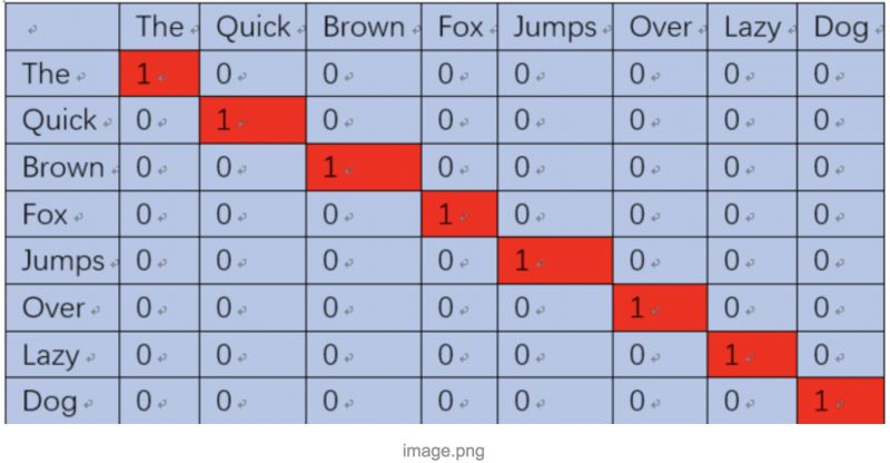
The word pair (the, quick) is represented as 【(1,0,0,0,0,0,0,0), (0,1,0,0,0,0,0,0)】
This way, it can be input into the neural network for training. When we input the word the into the neural network, we hope the network can also output an 8-dimensional vector, with the second dimension as close to 1 as possible and the others as close to 0.
This means we want the neural network to tell us that quick is more likely to appear around the word the. Of course, we also want the values of all positions in this 8-dimensional vector to sum to 1. WHY?
Because summing to 1 means that this 8-dimensional vector can be considered a probability distribution, which fits perfectly with our y value, which is also a probability distribution (one position is 1 and others are 0). We can use cross-entropy to measure the difference between the neural network’s output and our label y, thus defining the loss.
What? You don’t know what cross-entropy is? Please refer to my other article 【Machine Learning Interview: Various Confusing Entropies】; it should not disappoint you.
4Defining the Network Structure
From the previous discussion, we basically know what the neural network should look like. To summarize, we can determine the following:
-
The input to the neural network should be an 8-dimensional vector.
-
The neural network has only one hidden layer.
-
The output of the neural network should be an 8-dimensional vector, and the values of each dimension should sum to 1.
With this information, we can easily define the following network structure:
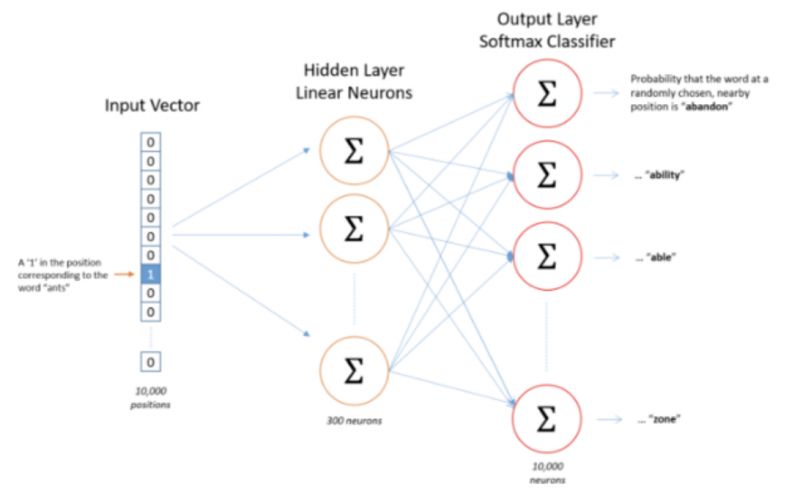
Observing this network structure, we can see that it does not have an activation function in the hidden layer, but the output layer uses softmax to ensure that the output vector is a probability distribution.
5Hidden Layer
Clearly, the output layer should have 8 neurons, allowing it to output an 8-dimensional vector. So how many neurons should the hidden layer have?
This depends on how many dimensions we want the word vectors to be. The number of hidden neurons will equal the dimensionality of the word vectors. Each hidden neuron receives an 8-dimensional vector as input. Suppose we have 3 hidden neurons (this is just for illustrative purposes; in practice, Google recommends 300, but the exact number should be determined through experimentation). Consequently, the weights of the hidden layer can be represented as an 8 by 3 matrix.
Now comes the moment of witnessing miracles!
After training is complete, each row of this 8 by 3 matrix is a word’s word vector! As shown in the following diagram:
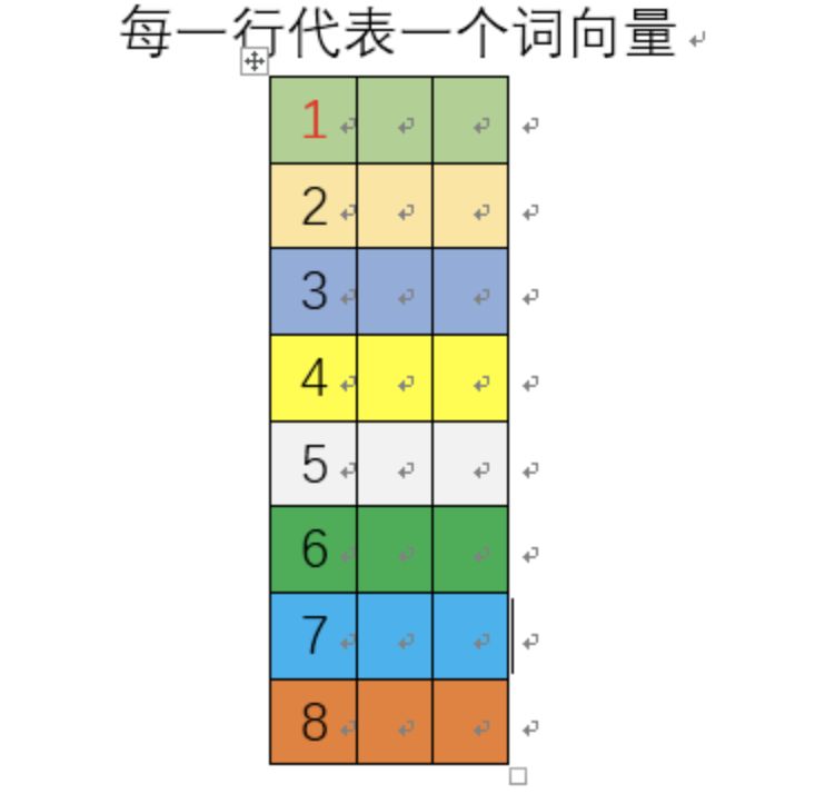
So, after training is complete, we only need to save the hidden layer’s weight matrix, as the output layer has already fulfilled its historical mission and can be discarded.
So how do we use the network after removing the output layer? We know that the input to the network is the one-hot encoded word, which, when multiplied by the hidden layer’s weight matrix, essentially retrieves the specific row of the weight matrix, as shown in the following diagram:
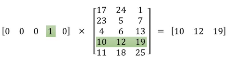
This means that the hidden layer effectively acts as a lookup table, with its output being the word vector of the input word.
6Output Layer
Once we obtain a word vector from the hidden layer, we need to go through the output layer. The number of neurons in the output layer is equal to the number of words in the corpus.
Each neuron can be considered to correspond to an output weight for a word, and multiplying the word vector by that output weight yields a number representing the likelihood of the corresponding word appearing around the input word. By applying softmax to the outputs of all output layer neurons, we can normalize the output into a probability distribution, as shown in the following diagram:
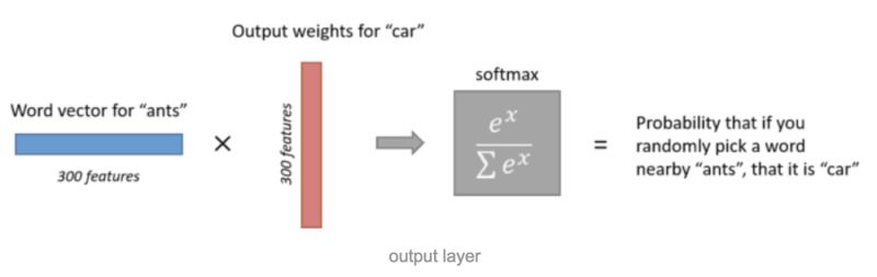
It is important to note that we say the output represents the probability of that word appearing around the input word; this “around” includes both the preceding and following words.
7Intuitive Insights
Earlier, we mentioned that the word vectors generated by the Skip-Gram algorithm can contain semantic information, meaning that semantically similar words will have similar word vectors. Here, we provide an intuitive explanation.
First, semantically similar words often have similar contexts. What does this mean? For example, the terms “smart” and “clever” are semantically similar, and their usage contexts are also similar; the words surrounding them are largely similar or the same.
Semantically similar words with similar contexts allow our neural network to produce similar output vectors during training for similar words. How does the network achieve this? The answer is that after training is complete, the network can generate similar word vectors for semantically similar words, as the output layer has already been trained and will not change.
This intuitive thinking is clearly not rigorous but provides good insight into neural networks.
Remember, Li Hongyi once said that someone asked why the LSTM design is so complex; how did the designer know that such a structure would achieve memory effects? In fact, it is not that they knew it would have memory effects; rather, they did it and then observed the effects. Doesn’t that feel a bit like the chicken or the egg? This is why deep learning is often referred to as a mystical science.
8Next Article Preview
You may have noticed that the neural network constructed by the Skip-Gram algorithm has too many neurons, resulting in a very large weight matrix. Suppose there are 10,000 words in our corpus, with generated word vectors of 300 dimensions.
Then the weight coefficients would be 10,000 * 300 * 2, which makes training such a large network very challenging. The next article will introduce some tips to help us reduce the training difficulty, making it feasible.

Recommended Reading:
When RNN Meets NER (Named Entity Recognition): Bidirectional LSTM, Conditional Random Fields (CRF), Stacked LSTM, Character Embeddings
[Deep Learning Practice] How to Handle RNN Input Variable-Length Sequences Padding in PyTorch
[Machine Learning Basic Theory] Detailed Explanation of Maximum A Posteriori Estimation (MAP)
Welcome to follow the official account for learning and communication~