

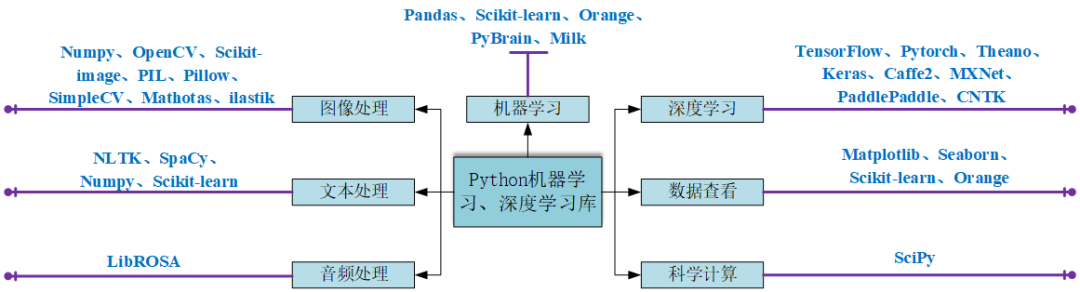
Approximately 8000 words, recommended reading time 15 minutes. This article provides a brief and comprehensive introduction to the currently more common artificial intelligence libraries.In order for everyone to have a preliminary understanding of commonly used Python libraries for artificial intelligence, to choose the libraries that can meet their needs for learning, a brief and comprehensive introduction to currently more common artificial intelligence libraries is provided.
1. Numpy
NumPy (Numerical Python) is an extension library for Python that supports a large number of dimensional arrays and matrix operations. In addition, it provides a large number of mathematical functions for array operations. NumPy is written in C language at the bottom, storing objects directly in arrays instead of storing object pointers, so its computational efficiency is much higher than pure Python code. We can compare the speed of calculating the sine values of a list between pure Python and using the Numpy library in the example:
import numpy as np
import math
import random
import time
start = time.time()
for i in range(10):
    list_1 = list(range(1,10000))
    for j in range(len(list_1)):
        list_1[j] = math.sin(list_1[j])
print("Using pure Python took {}s".format(time.time()-start))

start = time.time()
for i in range(10):
    list_1 = np.array(np.arange(1,10000))
    list_1 = np.sin(list_1)
print("Using Numpy took {}s".format(time.time()-start))
From the following running results, we can see that the speed of using the Numpy library is faster than the code written in pure Python:
Using pure Python took 0.017444372177124023s
Using Numpy took 0.001619577407836914s
2. OpenCV
OpenCV is a cross-platform computer vision library that can run on Linux, Windows, and Mac OS operating systems. It is lightweight and efficient, consisting of a series of C functions and a small number of C++ classes, while also providing a Python interface, implementing many common algorithms in image processing and computer vision. The following code attempts to use some simple filters, including image smoothing, Gaussian blur, etc.:
import numpy as np
import cv2 as cv
from matplotlib import pyplot as plt
img = cv.imread('h89817032p0.png')
kernel = np.ones((5,5),np.float32)/25
dst = cv.filter2D(img,-1,kernel)
blur_1 = cv.GaussianBlur(img,(5,5),0)
blur_2 = cv.bilateralFilter(img,9,75,75)
plt.figure(figsize=(10,10))
plt.subplot(221),plt.imshow(img[:,:,::-1]),plt.title('Original')
plt.xticks([]), plt.yticks([])
plt.subplot(222),plt.imshow(dst[:,:,::-1]),plt.title('Averaging')
plt.xticks([]), plt.yticks([])
plt.subplot(223),plt.imshow(blur_1[:,:,::-1]),plt.title('Gaussian')
plt.xticks([]), plt.yticks([])
plt.subplot(224),plt.imshow(blur_1[:,:,::-1]),plt.title('Bilateral')
plt.xticks([]), plt.yticks([])
plt.show()
OpenCV
3. Scikit-image
scikit-image is an image processing library based on scipy, which processes images as numpy arrays. For example, scikit-image can change the aspect ratio of images, and it provides functions such as rescale, resize, and downscale_local_mean.
from skimage import data, color, io
from skimage.transform import rescale, resize, downscale_local_mean

image = color.rgb2gray(io.imread('h89817032p0.png'))
image_rescaled = rescale(image, 0.25, anti_aliasing=False)
image_resized = resize(image, (image.shape[0] // 4, image.shape[1] // 4),
                      anti_aliasing=True)
image_downscaled = downscale_local_mean(image, (4, 3))
plt.figure(figsize=(20,20))
plt.subplot(221),plt.imshow(image, cmap='gray'),plt.title('Original')
plt.xticks([]), plt.yticks([])
plt.subplot(222),plt.imshow(image_rescaled, cmap='gray'),plt.title('Rescaled')
plt.xticks([]), plt.yticks([])
plt.subplot(223),plt.imshow(image_resized, cmap='gray'),plt.title('Resized')
plt.xticks([]), plt.yticks([])
plt.subplot(224),plt.imshow(image_downscaled, cmap='gray'),plt.title('Downscaled')
plt.xticks([]), plt.yticks([])
plt.show()
Scikit-image
4. PIL
The Python Imaging Library (PIL) has become the de facto standard library for image processing in Python, due to its powerful functionality and very simple API. However, since PIL only supports up to Python 2.7 and has not been maintained for years, a group of volunteers created a compatible version on the basis of PIL, called Pillow, which supports the latest Python 3.x and adds many new features. Therefore, we can skip PIL and directly install and use Pillow.
5. Pillow
Using Pillow to generate letter verification code images:
from PIL import Image, ImageDraw, ImageFont, ImageFilter
import random
# Random letter:
def rndChar():
    return chr(random.randint(65, 90))
# Random color 1:
def rndColor():
    return (random.randint(64, 255), random.randint(64, 255), random.randint(64, 255))
# Random color 2:
def rndColor2():
    return (random.randint(32, 127), random.randint(32, 127), random.randint(32, 127))
# 240 x 60:
width = 60 * 6
height = 60 * 6
image = Image.new('RGB', (width, height), (255, 255, 255))
# Create Font object:
font = ImageFont.truetype('/usr/share/fonts/wps-office/simhei.ttf', 60)
# Create Draw object:
draw = ImageDraw.Draw(image)
# Fill each pixel:
for x in range(width):
    for y in range(height):
        draw.point((x, y), fill=rndColor())
# Output text:
for t in range(6):
    draw.text((60 * t + 10, 150), rndChar(), font=font, fill=rndColor2())
# Blur:
image = image.filter(ImageFilter.BLUR)
image.save('code.jpg', 'jpeg')
Verification Code
6. SimpleCV
SimpleCV is an open-source framework for building computer vision applications. Using it, one can access high-performance computer vision libraries like OpenCV without having to first understand terms like bit depth, file formats, color spaces, buffer management, features, or matrices. However, its support for Python 3 is very poor, and using the following code in Python 3.7:
from SimpleCV import Image, Color, Display
# load an image from imgur
img = Image('http://i.imgur.com/lfAeZ4n.png')
# use a keypoint detector to find areas of interest
feats = img.findKeypoints()
# draw the list of keypoints
feats.draw(color=Color.RED)
# show the resulting image.
img.show()
# apply the stuff we found to the image.
output = img.applyLayers()
# save the results.
output.save('juniperfeats.png')
Will report the following error, so it is not recommended to use in Python 3:
SyntaxError: Missing parentheses in call to 'print'. Did you mean print('unit test')?7. Mahotas
Mahotas is a fast computer vision algorithm library built on top of Numpy, currently having over 100 image processing and computer vision functions, and is continuously growing. Using Mahotas to load images and manipulate pixels:
import numpy as np
import mahotas
import mahotas.demos
from mahotas.thresholding import soft_threshold
from matplotlib import pyplot as plt
from os import path
f = mahotas.demos.load('lena', as_grey=True)
f = f[128:,128:]
plt.gray()
# Show the data:
print("Fraction of zeros in original image: {0}".format(np.mean(f==0)))
plt.imshow(f)
plt.show()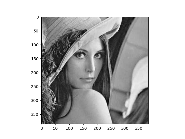 Mahotas
8. Ilastik
Ilastik provides users with good machine learning-based bioinformatics image analysis services, allowing easy segmentation, classification, tracking, and counting of cells or other experimental data using machine learning algorithms. Most operations are interactive and do not require expertise in machine learning.
9. Scikit-Learn
Scikit-learn is a free software machine learning library for the Python programming language. It has a variety of classification, regression, and clustering algorithms, including support vector machines, random forests, gradient boosting, k-means, and DBSCAN. Implementing the KMeans algorithm using Scikit-learn:
import time
import numpy as np
import matplotlib.pyplot as plt
from sklearn.cluster import MiniBatchKMeans, KMeans
from sklearn.metrics.pairwise import pairwise_distances_argmin
from sklearn.datasets import make_blobs
# Generate sample data
np.random.seed(0)
batch_size = 45
centers = [[1, 1], [-1, -1], [1, -1]]
n_clusters = len(centers)
X, labels_true = make_blobs(n_samples=3000, centers=centers, cluster_std=0.7)
# Compute clustering with KMeans
k_means = KMeans(init='k-means++', n_clusters=3, n_init=10)
t0 = time.time()
k_means.fit(X)
t_batch = time.time() - t0
# Compute clustering with MiniBatchKMeans
mbk = MiniBatchKMeans(init='k-means++', n_clusters=3, batch_size=batch_size,
                      n_init=10, max_no_improvement=10, verbose=0)
t0 = time.time()
mbk.fit(X)
t_mini_batch = time.time() - t0
# Plot result
fig = plt.figure(figsize=(8, 3))
fig.subplots_adjust(left=0.02, right=0.98, bottom=0.05, top=0.9)
colors = ['#4EACC5', '#FF9C34', '#4E9A06']
# We want to have the same colors for the same cluster from the
# MiniBatchKMeans and the KMeans algorithm. Let's pair the cluster centers per
# closest one.
k_means_cluster_centers = k_means.cluster_centers_
order = pairwise_distances_argmin(k_means.cluster_centers_,
                                  mbk.cluster_centers_)
mbk_means_cluster_centers = mbk.cluster_centers_[order]
k_means_labels = pairwise_distances_argmin(X, k_means_cluster_centers)
mbk_means_labels = pairwise_distances_argmin(X, mbk_means_cluster_centers)
# KMeans
for k, col in zip(range(n_clusters), colors):
    my_members = k_means_labels == k
    cluster_center = k_means_cluster_centers[k]
    plt.plot(X[my_members, 0], X[my_members, 1], 'w',
            markerfacecolor=col, marker='.')
    plt.plot(cluster_center[0], cluster_center[1], 'o', markerfacecolor=col,
            markeredgecolor='k', markersize=6)
plt.title('KMeans')
plt.xticks(())
plt.yticks(())
plt.show()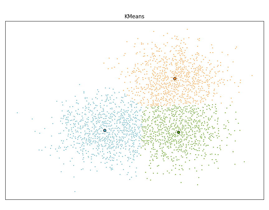
10. SciPy
The SciPy library provides many user-friendly and efficient numerical computations, such as numerical integration, interpolation, optimization, linear algebra, etc. The SciPy library defines many special functions in mathematical physics, including elliptical functions, Bessel functions, gamma functions, beta functions, hypergeometric functions, parabolic cylinder functions, and so on.
from scipy import special
import matplotlib.pyplot as plt
import numpy as np

def drumhead_height(n, k, distance, angle, t):
    kth_zero = special.jn_zeros(n, k)[-1]
    return np.cos(t) * np.cos(n*angle) * special.jn(n, distance*kth_zero)

theta = np.r_[0:2*np.pi:50j]
radius = np.r_[0:1:50j]
x = np.array([r * np.cos(theta) for r in radius])
y = np.array([r * np.sin(theta) for r in radius])
z = np.array([drumhead_height(1, 1, r, theta, 0.5) for r in radius])

fig = plt.figure()
ax = fig.add_axes(rect=(0, 0.05, 0.95, 0.95), projection='3d')
ax.plot_surface(x, y, z, rstride=1, cstride=1, cmap='RdBu_r', vmin=-0.5, vmax=0.5)
ax.set_xlabel('X')
ax.set_ylabel('Y')
ax.set_xticks(np.arange(-1, 1.1, 0.5))
ax.set_yticks(np.arange(-1, 1.1, 0.5))
ax.set_zlabel('Z')
plt.show()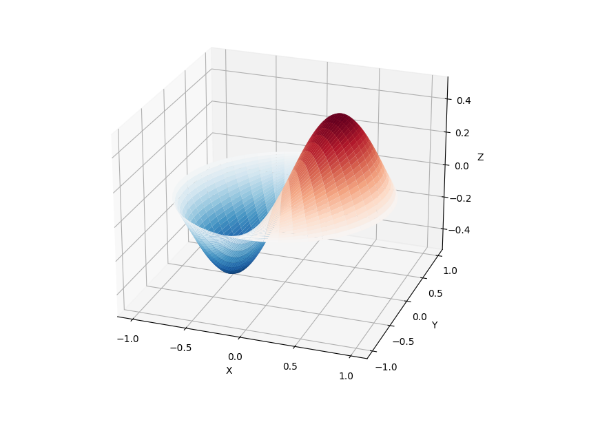
11. NLTK
NLTK is a library for building Python programs to work with human language data. It provides easy-to-use interfaces to over 50 corpora and lexical resources (such as WordNet), as well as a suite of text processing libraries for classification, tokenization, stemming, tagging, parsing, and semantic reasoning, and is often referred to as “a wonderful tool for teaching, and working in, computational linguistics using Python.”
import nltk
from nltk.corpus import treebank
# First time use requires downloading
nltk.download('punkt')
nltk.download('averaged_perceptron_tagger')
nltk.download('maxent_ne_chunker')
nltk.download('words')
nltk.download('treebank')

sentence = "At eight o'clock on Thursday morning Arthur didn't feel very good."
# Tokenize
tokens = nltk.word_tokenize(sentence)
tagged = nltk.pos_tag(tokens)
# Identify named entities
entities = nltk.chunk.ne_chunk(tagged)
# Display a parse tree
t = treebank.parsed_sents('wsj_0001.mrg')[0]
t.draw()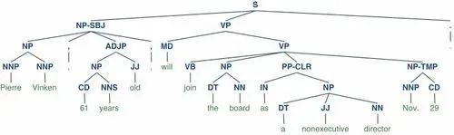
12. spaCy
spaCy is a free open-source library for advanced NLP in Python. It can be used to build applications that process large amounts of text; it can also be used to build information extraction or natural language understanding systems, or to preprocess text for deep learning.
import spacy
texts = [
    "Net income was $9.4 million compared to the prior year of $2.7 million.",
    "Revenue exceeded twelve billion dollars, with a loss of $1b.",
]

nlp = spacy.load("en_core_web_sm")
for doc in nlp.pipe(texts, disable=["tok2vec", "tagger", "parser", "attribute_ruler", "lemmatizer"]):
    # Do something with the doc here
    print([(ent.text, ent.label_) for ent in doc.ents])
nlp.pipe generates Doc objects, allowing us to iterate over them and access named entity predictions:
[('$9.4 million', 'MONEY'), ('the prior year', 'DATE'), ('$2.7 million', 'MONEY')]
[('twelve billion dollars', 'MONEY'), ('1b', 'MONEY')]
13. LibROSA
librosa is a Python library for music and audio analysis that provides the necessary functions and features to create music information retrieval systems.
# Beat tracking example
import librosa
# 1. Get the file path to an included audio example
filename = librosa.example('nutcracker')
# 2. Load the audio as a waveform `y`
#    Store the sampling rate as `sr`
y, sr = librosa.load(filename)
# 3. Run the default beat tracker
tempo, beat_frames = librosa.beat.beat_track(y=y, sr=sr)
print('Estimated tempo: {:.2f} beats per minute'.format(tempo))
# 4. Convert the frame indices of beat events into timestamps
beat_times = librosa.frames_to_time(beat_frames, sr=sr)
14. Pandas
Pandas is a fast, powerful, flexible, and easy-to-use open-source data analysis and manipulation tool. Pandas can import data from various file formats such as CSV, JSON, SQL, and Microsoft Excel, and can perform operations on various data, such as merging, reshaping, selecting, as well as data cleaning and feature engineering. Pandas is widely used in academic, financial, statistical, and various data analysis fields.
import matplotlib.pyplot as plt
import pandas as pd
import numpy as np

ts = pd.Series(np.random.randn(1000), index=pd.date_range("1/1/2000", periods=1000))
ts = ts.cumsum()
df = pd.DataFrame(np.random.randn(1000, 4), index=ts.index, columns=list("ABCD"))
df = df.cumsum()
df.plot()
plt.show()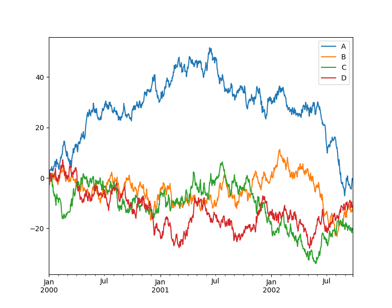
15. Matplotlib
Matplotlib is a plotting library for Python that provides a complete set of command APIs similar to MATLAB, allowing the generation of publication-quality beautiful graphics. Matplotlib makes plotting very simple, achieving an excellent balance between usability and performance. Using Matplotlib to plot multiple curves:
# plot_multi_curve.py
import numpy as np
import matplotlib.pyplot as plt
x = np.linspace(0.1, 2 * np.pi, 100)
y_1 = x
y_2 = np.square(x)
y_3 = np.log(x)
y_4 = np.sin(x)
plt.plot(x,y_1)
plt.plot(x,y_2)
plt.plot(x,y_3)
plt.plot(x,y_4)
plt.show()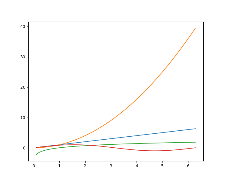 Matplotlib
16. Seaborn
Seaborn is a Python data visualization library that provides a higher-level API encapsulation based on Matplotlib, making plotting easier. Seaborn should be seen as a complement to Matplotlib, rather than a replacement.
import seaborn as sns
import matplotlib.pyplot as plt
sns.set_theme(style="ticks")
df = sns.load_dataset("penguins")
sns.pairplot(df, hue="species")
plt.show()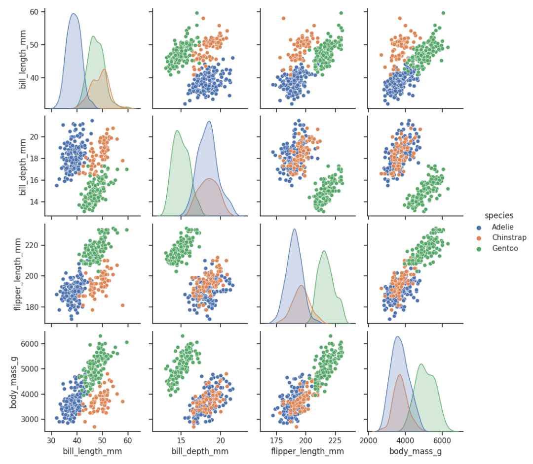
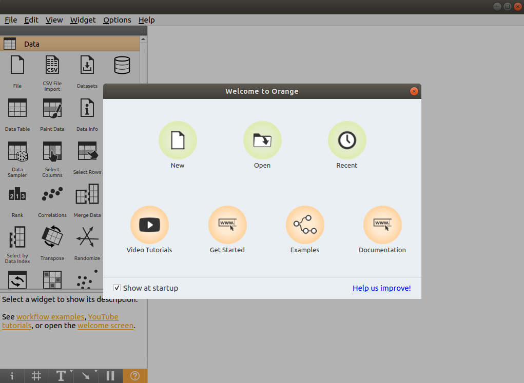
17. Orange
Orange is an open-source data mining and machine learning software that provides a range of data exploration, visualization, preprocessing, and modeling components. Orange has a beautiful and intuitive interactive user interface, making it very suitable for beginners to perform exploratory data analysis and visualization; at the same time, advanced users can also use it as a programming module in Python for data manipulation and component development. You can install Orange using pip, and it has received positive reviews.
$ pip install orange3After installation, enter the orange-canvas command in the command line to start the Orange graphical interface:
$ orange-canvasOnce started, you will see the Orange graphical interface for various operations.
18. PyBrain
PyBrain is a modular machine learning library for Python. Its goal is to provide flexible, easy-to-use, and powerful algorithms for machine learning tasks and various predefined environments to test and compare algorithms. PyBrain is an abbreviation for Python-Based Reinforcement Learning, Artificial Intelligence, and Neural Network Library. We will use a simple example to demonstrate the usage of PyBrain by building a Multi-Layer Perceptron (MLP). First, we create a new feedforward network object:
from pybrain.structure import FeedForwardNetwork
n = FeedForwardNetwork()
Next, build the input, hidden, and output layers:
from pybrain.structure import LinearLayer, SigmoidLayer
inLayer = LinearLayer(2)
hiddenLayer = SigmoidLayer(3)
outLayer = LinearLayer(1)
To use the constructed layers, they must be added to the network:
n.addInputModule(inLayer)
n.addModule(hiddenLayer)
n.addOutputModule(outLayer)
Multiple input and output modules can be added. To perform forward computation and backpropagation, the network must know which layers are input and which layers are output. This requires explicitly defining how they should connect. For this, we use the most common connection type, a fully connected layer, implemented by the FullConnection class:
from pybrain.structure import FullConnection
in_to_hidden = FullConnection(inLayer, hiddenLayer)
hidden_to_out = FullConnection(hiddenLayer, outLayer)
Like layers, we must explicitly add them to the network:
n.addConnection(in_to_hidden)
n.addConnection(hidden_to_out)
All elements are now ready, and finally, we need to call the .sortModules() method to make the MLP available:
n.sortModules()This call performs some internal initialization that is necessary before using the network.
19. Milk
MILK (MACHINE LEARNING TOOLKIT) is a machine learning toolkit for the Python language. It mainly includes many classifiers such as SVMs, K-NN, random forests, and decision trees using supervised classification methods. It can also perform feature selection and form different classification systems such as unsupervised learning, close relationship propagation, and K-means clustering supported by MILK. Training a classifier using MILK:
import numpy as np
import milk
features = np.random.rand(100,10)
labels = np.zeros(100)
features[50:] += .5
labels[50:] = 1
learner = milk.defaultclassifier()
model = learner.train(features, labels)
# Now you can use the model on new examples:
example = np.random.rand(10)
print(model.apply(example))
example2 = np.random.rand(10)
example2 += .5
print(model.apply(example2))
20. TensorFlow
TensorFlow is an end-to-end open-source machine learning platform. It has a comprehensive and flexible ecosystem, generally divided into TensorFlow 1.x and TensorFlow 2.x. The main difference between TensorFlow 1.x and TensorFlow 2.x is that TF 1.x uses static graphs while TF 2.x uses eager mode dynamic graphs. Here, TensorFlow 2.x is mainly used as an example to demonstrate how to build a convolutional neural network (CNN) in TensorFlow 2.x.
import tensorflow as tf
from tensorflow.keras import datasets, layers, models
# Data loading
(train_images, train_labels), (test_images, test_labels) = datasets.cifar10.load_data()
# Data preprocessing
train_images, test_images = train_images / 255.0, test_images / 255.0
# Model building
model = models.Sequential()
model.add(layers.Conv2D(32, (3, 3), activation='relu', input_shape=(32, 32, 3)))
model.add(layers.MaxPooling2D((2, 2)))
model.add(layers.Conv2D(64, (3, 3), activation='relu'))
model.add(layers.MaxPooling2D((2, 2)))
model.add(layers.Conv2D(64, (3, 3), activation='relu'))
model.add(layers.Flatten())
model.add(layers.Dense(64, activation='relu'))
model.add(layers.Dense(10))
# Model compilation and training
model.compile(optimizer='adam',
              loss=tf.keras.losses.SparseCategoricalCrossentropy(from_logits=True),
              metrics=['accuracy'])
history = model.fit(train_images, train_labels, epochs=10,
                     validation_data=(test_images, test_labels))
21. PyTorch
PyTorch is the predecessor of Torch, with the same underlying framework as Torch, but many parts rewritten in Python, making it more flexible and supporting dynamic graphs, while providing a Python interface.
# Import libraries
import torch
from torch import nn
from torch.utils.data import DataLoader
from torchvision import datasets
from torchvision.transforms import ToTensor, Lambda, Compose
import matplotlib.pyplot as plt
# Model building
device = "cuda" if torch.cuda.is_available() else "cpu"
print("Using {} device".format(device))
# Define model
class NeuralNetwork(nn.Module):
    def __init__(self):
        super(NeuralNetwork, self).__init__()
        self.flatten = nn.Flatten()
        self.linear_relu_stack = nn.Sequential(
            nn.Linear(28*28, 512),
            nn.ReLU(),
            nn.Linear(512, 512),
            nn.ReLU(),
            nn.Linear(512, 10),
            nn.ReLU()
        )
    def forward(self, x):
        x = self.flatten(x)
        logits = self.linear_relu_stack(x)
        return logits
model = NeuralNetwork().to(device)
# Loss function and optimizer
loss_fn = nn.CrossEntropyLoss()
optimizer = torch.optim.SGD(model.parameters(), lr=1e-3)
# Model training
def train(dataloader, model, loss_fn, optimizer):
    size = len(dataloader.dataset)
    for batch, (X, y) in enumerate(dataloader):
        X, y = X.to(device), y.to(device)
        # Compute prediction error
        pred = model(X)
        loss = loss_fn(pred, y)
        # Backpropagation
        optimizer.zero_grad()
        loss.backward()
        optimizer.step()
        if batch % 100 == 0:
            loss, current = loss.item(), batch * len(X)
            print(f"loss: {loss:>7f}  [{current:>5d}/{size:>5d}]")
22. Theano
Theano is a Python library that allows the definition, optimization, and efficient computation of mathematical expressions involving multidimensional arrays, built on top of NumPy. Implementing the computation of the Jacobian matrix in Theano:
import theano
import theano.tensor as T
x = T.dvector('x')
y = x ** 2
J, updates = theano.scan(lambda i, y,x : T.grad(y[i], x), sequences=T.arange(y.shape[0]), non_sequences=[y,x])
f = theano.function([x], J, updates=updates)
f([4, 4])
23. Keras
Keras is a high-level neural networks API written in Python that can run on top of TensorFlow, CNTK, or Theano. The development focus of Keras is to support fast experimentation, allowing ideas to be translated into results with minimal delay.
from keras.models import Sequential
from keras.layers import Dense
# Model building
model = Sequential()
model.add(Dense(units=64, activation='relu', input_dim=100))
model.add(Dense(units=10, activation='softmax'))
# Model compilation and training
model.compile(loss='categorical_crossentropy',
              optimizer='sgd',
              metrics=['accuracy'])
model.fit(x_train, y_train, epochs=5, batch_size=32)
24. Caffe
On the official Caffe2 website, it is stated: Caffe2 is now part of PyTorch. While these APIs will continue to work, users are encouraged to use PyTorch APIs.
25. MXNet
MXNet is a deep learning framework designed for efficiency and flexibility. It allows for a mix of symbolic programming and imperative programming to maximize efficiency and productivity. Building a handwritten digit recognition model using MXNet:
import mxnet as mx
from mxnet import gluon
from mxnet.gluon import nn
from mxnet import autograd as ag
import mxnet.ndarray as F
# Data loading
mnist = mx.test_utils.get_mnist()
batch_size = 100
train_data = mx.io.NDArrayIter(mnist['train_data'], mnist['train_label'], batch_size, shuffle=True)
val_data = mx.io.NDArrayIter(mnist['test_data'], mnist['test_label'], batch_size)
# CNN model
class Net(gluon.Block):
    def __init__(self, **kwargs):
        super(Net, self).__init__(**kwargs)
        self.conv1 = nn.Conv2D(20, kernel_size=(5,5))
        self.pool1 = nn.MaxPool2D(pool_size=(2,2), strides = (2,2))
        self.conv2 = nn.Conv2D(50, kernel_size=(5,5))
        self.pool2 = nn.MaxPool2D(pool_size=(2,2), strides = (2,2))
        self.fc1 = nn.Dense(500)
        self.fc2 = nn.Dense(10)
    def forward(self, x):
        x = self.pool1(F.tanh(self.conv1(x)))
        x = self.pool2(F.tanh(self.conv2(x)))
        # 0 means copy over size from corresponding dimension.
        # -1 means infer size from the rest of dimensions.
        x = x.reshape((0, -1))
        x = F.tanh(self.fc1(x))
        x = F.tanh(self.fc2(x))
        return x
net = Net()
# Initialize and define optimizer
# set the context on GPU is available otherwise CPU
ctx = [mx.gpu() if mx.test_utils.list_gpus() else mx.cpu()]
net.initialize(mx.init.Xavier(magnitude=2.24), ctx=ctx)
trainer = gluon.Trainer(net.collect_params(), 'sgd', {'learning_rate': 0.03})
# Model training
# Use Accuracy as the evaluation metric.
metric = mx.metric.Accuracy()
softmax_cross_entropy_loss = gluon.loss.SoftmaxCrossEntropyLoss()
for i in range(epoch):
    # Reset the train data iterator.
    train_data.reset()
    for batch in train_data:
        data = gluon.utils.split_and_load(batch.data[0], ctx_list=ctx, batch_axis=0)
        label = gluon.utils.split_and_load(batch.label[0], ctx_list=ctx, batch_axis=0)
        outputs = []
        # Inside training scope
        with ag.record():
            for x, y in zip(data, label):
                z = net(x)
                # Computes softmax cross entropy loss.
                loss = softmax_cross_entropy_loss(z, y)
                # Backpropogate the error for one iteration.
                loss.backward()
                outputs.append(z)
        metric.update(label, outputs)
        trainer.step(batch.data[0].shape[0])
    # Gets the evaluation result.
    name, acc = metric.get()
    # Reset evaluation result to initial state.
    metric.reset()
    print('training acc at epoch %d: %s=%f'%(i, name, acc))
26. PaddlePaddle
PaddlePaddle is based on Baidu’s years of deep learning technology research and business applications, integrating deep learning core training and inference frameworks, basic model libraries, end-to-end development kits, and rich tool components. It is China’s first independently developed, fully functional, open-source industrial-grade deep learning platform. Implementing LeNet5 using PaddlePaddle:
# Import necessary packages
import paddle
import numpy as np
from paddle.nn import Conv2D, MaxPool2D, Linear
## Network construction
import paddle.nn.functional as F
# Define LeNet network structure
class LeNet(paddle.nn.Layer):
    def __init__(self, num_classes=1):
        super(LeNet, self).__init__()
        # Create convolutional and pooling layers
        # Create the first convolutional layer
        self.conv1 = Conv2D(in_channels=1, out_channels=6, kernel_size=5)
        self.max_pool1 = MaxPool2D(kernel_size=2, stride=2)
        # Logical dimension: pooling layer does not change the number of channels; current number of channels is 6
        # Create the second convolutional layer
        self.conv2 = Conv2D(in_channels=6, out_channels=16, kernel_size=5)
        self.max_pool2 = MaxPool2D(kernel_size=2, stride=2)
        # Create the third convolutional layer
        self.conv3 = Conv2D(in_channels=16, out_channels=120, kernel_size=4)
        # Logical dimension: input layer flattens data [B,C,H,W] -> [B,C*H*W]
        # Input size is [28,28], after three convolutions and two poolings, C*H*W equals 120
        self.fc1 = Linear(in_features=120, out_features=64)
        # Create fully connected layers, the number of output neurons for the first fully connected layer is 64, the number of output neurons for the second fully connected layer is the number of classification labels
        self.fc2 = Linear(in_features=64, out_features=num_classes)
    # Forward computation process of the network
    def forward(self, x):
        x = self.conv1(x)
        # Each convolutional layer uses the sigmoid activation function, followed by a 2x2 pooling
        x = F.sigmoid(x)
        x = self.max_pool1(x)
        x = F.sigmoid(x)
        x = self.conv2(x)
        x = self.max_pool2(x)
        x = self.conv3(x)
        # Logical dimension: input layer flattens data [B,C,H,W] -> [B,C*H*W]
        x = paddle.reshape(x, [x.shape[0], -1])
        x = self.fc1(x)
        x = F.sigmoid(x)
        x = self.fc2(x)
        return x
27. CNTK
CNTK (Cognitive Toolkit) is a deep learning toolkit that describes neural networks as a series of computational steps through directed graphs. In this directed graph, leaf nodes represent input values or network parameters, while other nodes represent matrix operations on their inputs. CNTK can easily implement and combine popular model types such as CNNs, etc. CNTK describes a neural network using network description language (NDL). Simply put, it describes the input features, input labels, some parameters, the computation relationships between parameters and inputs, and what the target nodes are.
NDLNetworkBuilder=[
        run=ndlLR
        ndlLR=[
      # sample and label dimensions
      SDim=$dimension$
      LDim=1
          features=Input(SDim, 1)
          labels=Input(LDim, 1)
          # parameters to learn
          B0 = Parameter(4)
          W0 = Parameter(4, SDim)
                  B = Parameter(LDim)
          W = Parameter(LDim, 4)
          # operations
          t0 = Times(W0, features)
          z0 = Plus(t0, B0)
          s0 = Sigmoid(z0)
               t = Times(W, s0)
          z = Plus(t, B)
          s = Sigmoid(z)
              LR = Logistic(labels, s)
          EP = SquareError(labels, s)
          # root nodes
          FeatureNodes=(features)
          LabelNodes=(labels)
          CriteriaNodes=(LR)
          EvalNodes=(EP)
          OutputNodes=(s,t,z,s0,W0)
    ]
Edited by: Yu Tengkai
Proofread by: Lin Yilin